Toys for Billionaires: Sports Franchises as Trophy Assets!

I have always loved sports, playing tennis and cricket when I was growing up, before transitioning to fan status, cheering for my favored teams from the sidelines. I also like finance, perhaps not as much as sports, but there are winners and losers in the investment game as well. Thus, it should come as no surprise that when the two connect, as is the case when teams are bought and sold, or players are signed, I am doubly interested. The time is ripe now to talk about how professional sports, in its many variations around the world, has blown a financial gasket, as you see teams sold for prices that seem out of sync with their financial fundamentals and players signed on contracts that equate to the GDP of a small country. In this post, that is my objective, and if get sidetracked, as a sports fans, I apologize in advance.

The Lead In

    In its idealistic form, sports is about competition and the human spirit, and is divorced from money. That was the ideal behind not just the Olympic ban on athletes from being paid for performing, but also behind major tennis tournaments being restricted to just amateurs until 1968 and the entire collegiate sports scene. Both restrictions eventually fell, weighted down by hypocrisy, since the same entities that preached the importance of keeping money out of sports, and insisted that the players on the field could not make a living from playing it, engorged themselves on its monetary spoils. At this point, it seems undeniable that sports and money are entwined, and that trying to separate the two is pointless.

The Story Lines

    As the walls between sports and money have crumbled, we have become used to seeing mind-boggling numbers on sports transactions, whether it be in the form on broadcasting networks paying for the rights to carry sporting events or player contracts pushing into the hundreds of millions. Even by those standards, though, the last few months have delivered surprises that have staggered even the most jaded sports-watchers:

• Player contracts: While player contracts have become bigger over time, the $776 million offer by Al-Hilal, a Saudi team, to Kylian Mbappe, the French superstar on contract with PSG, for a one-year contract to play with the team was eye-popping in magnitude. While Mbappe turned down the offer and is considering a ten-year deal with PSG, the numbers involved in the Al-Hilal deal are almost impossible to justify on purely economic terms. In parallel, as the 2023 baseball season winds down, questions about which team would sign Shohei Ohtani, its best player, and for how much were widely debated in the media.
• Sports franchise transactions: In 2023, the Washington Commanders, an NFL team with a decidedly mixed record on the field and a history of controversy around its name and owner, was sold for over $6 billion to a consortium, making it the highest priced sports franchise transaction in history. It followed a decade or more of ever-rising prices for sports franchises around the world, from the Premier League (soccer) in the UK, to the IPL (cricket) and across professional sports in the US. 
• Sport disruptions: The last year has also brought threats to sports franchises, striking at their very existence. The Saudi team bid for Mbappe reflected a broader attempt by the country to disrupt professional sports, with professional golf, in particular, in the cross hairs. When LIV made its bid by signing up some of the best-known golf players in the world to play in its tournaments,  few gave it a chance of success against the PGA, but in 2023, it was the PGA that conceded the fight in the money game.
• Broadcasting upheaval: As the revenues from sports has shifted from the playing fields to media, it is the size of the media contracts that determine how lucrative a sport is. In 2021, we saw the NFL, the richest franchise in the world, enter into new media contracts to cover the next decade of broadcasting rights for the sport. These contracts are not only expected to bring in a staggering $114 billion in revenues to the NFL in the next decade, but in a reflection of the times, they are split among four different broadcasters (ESPN, CBS, NBC and Fox), with Amazon Prime picking up the slack. The increasing importance of streaming in the media business was illustrated when the IPL, India’s cricket league, sold its media rights for the next five years for television broadcasting to Star India, a Disney-owned subsidiary, for roughly $3 billion, and the streaming rights for the same period to Viacom18, a Reliance-controlled joint venture, for about the same amount.

While these stories cover disparate parts of sports, and the only thing they share in common is the explosively large financial numbers, I will argue, in this post, that they represent an acceleration in a phenomenon that will change how these sports will get played and watched.

Rising Franchise Prices

    Even a casual follower of the news on sports franchises changing hands, no matter what the sport, must have noticed the surge in the pricing of sports franchises, with little or no obvious connection to team success on the field; the Washington Commanders, the target of $6 billion acquisition, have won 63 games, while losing 97, in the last decade. In fact, the five highest prices paid for sports teams have all be paid in the last two years, as can be seen in the list of ten most expensive sports franchise transactions in history:

Team	League	Year	Price (in $ billions)
Washington Commanders	NFL	2023	$6.05
Chelsea	Premier League	2022	$5.30
Denver Broncos	NFL	2022	$4.70
Phoenix Suns	NBA	2023	$4.00
Milwaukee Bucks	NBA	2023	$3.50
New York Mets	MLB	2020	$2.40
Brooklyn Nets	NBA	2019	$2.40
Carolina Panthers	NFL	2018	$2.20
Houston Rockets	NBA	2017	$2.20
Los Angeles Dodgers	MLB	2012	$2.00

These high prices, though, represent the continuation of a trend that we have seen over the last few decades in franchise pricing, with the graph below looking at every major sports transaction between 1998 and 2023:

As you can see, transaction prices for sports franchises have been marching upwards for the last two decades, with NBA and NFL teams registering the biggest increases, but have seen breakaway surges in the last few years.

    Some of you may be familiar with the Forbes annual listings of the most valuable teams in the world, and you may have wondered how they value sports teams. The truth, and I will clarify what I mean shortly, is that Forbes does not value sports franchises, but prices them. Since Forbes gets draws on actual transaction prices as guidance in their estimates, the pricing that Forbes attaches to teams has risen with transaction prices. In the graph below, for instance, I report the cumulative pricing of all NFL teams, as estimated by Forbes, from 2012 to 2022:

The collective pricing of all NFL teams, according to Forbes, has risen from  $37.6 billion in 2012 to $132.5 billion in 2022. In fact, I will be willing to predict that given the Washington Commanders transaction, the pricing of every NFL team on the Forbes list will be higher in 2023.

    With the pricing process in mind, it is instructive to look at the collective pricing, in millions of US dollars, of global sports franchises, as of the most recent updates from 2022 and 2023:

	Cumulative Pricing (in $ mil)	Highest Priced	Lowest Priced
NFL (US Football)	$132,500	$7,640	$4,140
NBA (Basketball)	$85,910	$7,000	$1,600
MLB (Baseball)	$69,550	$7,100	$1,000
NHL (Hockey)	$32,350	$2,200	$450
MLS (US Soccer)	$16,200	$1,000	$350
Premier League (To 20)	$30,255	$5,950	$145
IPL (Indian Cricket)	$10,430	$1,300	$850

The NFL is the most valuable franchise in the world, in terms of collective pricing of all of its teams, followed by basketball and baseball. The collective pricing of all soccer teams around the world may actually be close to or even exceed the pricing of baseball or basketball teams, but just the top 20 Premier League teams have a pricing of about $30 billion. The ten teams that comprise the IPL, the Indian cricket league, have a collective pricing in excess of $10 billion. One interesting difference across franchises is the differences between the highest and lowest priced franchises, with the NFL having the smallest difference, and we will talk about how the way broadcasting revenue are shared can explain this divergence across sports franchises.

    Finally, there is a subset of sports franchises that are publicly traded, but it is a very small one. Among US sports franchises, the one that comes closes is Madison Square Garden Sports, which in addition to owning the arena (Madison Square Garden) also owns the New York Knicks (NBA) and the New York Rangers (hockey), but it is closely held, with the Dolan family firmly in control. Outside of the US, Manchester United is the highest-profile example of a publicly traded company, but it too is closely held, with control in the hands of the Glazer family. There are a few European soccer teams that are publicly traded, but they all tend to be closely held, with light liquidity. 

Price vs Value

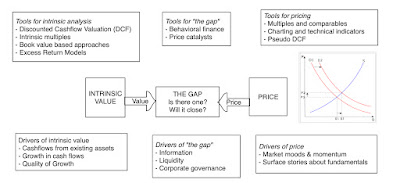
    If you find me finicky, when I label the Forbes estimates for franchises as prices, rather than values, it is best understood by contrasting price and value, two words that, at least to me, mean very different things and require different mindsets:

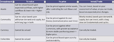
As you can see from the picture, while value is driven by familiar fundamentals (cash flows, growth and risk), price is determined by demand and supply, which, in turn, are driven by mood and momentum, behavioral factors that don’t play a key role in determining value. I used this contrast, a few years ago, to classify investments and talk about price and value with each one:

As you can see, collectibles and currencies can only be priced, and while commodities may have an aggregate fundamental value, they are more likely to be  priced than valued. It is only with assets that are expected to generate cashflows in the future that value even comes into play. A company or a business can be valued, and that value will reflect its capacity to generate cash flows in the future, but it can also be priced, based upon what others are paying for similar companies. In fact, almost every investment philosophy can be framed in terms of whether you believe that there can be a gap between value and price, and when there is a gap, how quickly it will cause, as well as catalyst that cause that closing.

    There is a sub-grouping of assets, though, that is worth carving out and considering differently, and I will call these trophy assets. A trophy asset has expected cash flows, and can be valued like any other asset, but the people who buy it often do so, less for its asset status and more as a collectible. Powered by emotional factors, the prices of trophy assets can rise above values and stay higher, since, unlike other assets, there is no catalyst that will cause the gap between price and value to close. So, what is it that makes it for a "trophy assets"?

1. Emotional appeal overwhelms financial characteristics: The key to a trophy asset is that the core of its attraction, to potential buyers or investors, lies less in business models and cash flows, and more in the emotional appeal it has to buyers. That appeal may be only to a subset of individuals, but these buyers want to own the asset more for the emotional dividends, not the cashflows.
2. It is unique: Trophy assets pack a punch because they are unique, insofar as they cannot be replicated by someone, even if that someone has substantial financial resources.
3. It is scarce: For trophy assets to command a pricing that is significantly higher than value, they have to be scarce.
4. It is bought and held for non-financial reasons: If trophy assets are opened up for bidding, the winning bidder will almost always be an individual or entity that is buying the asset more for its history or provenance, not its financial characteristics.

Examples of trophy assets can range the spectrum from legendary real estate properties, such as the Ritz Carlton in London, to publications like the Economist or the Financial Times. 

    Once an asset crosses the threshold to trophy status, you can expect the following to occur. First, it will look over priced, relative to financial fundamentals (earnings, revenues, cash flows), and relative to peer group assets that do not enjoy the same trophy status. Second, and this is critical, even as price increases relative to value, the mechanism that causes the gap to close, often stemming from a recognition that the you have paid too much for something, given its capacity to generate earnings and cash flows, will stop working. After all, if buyers price trophy assets based upon their emotional connections, they are entering the transaction, knowing that they have paid too much, and do not care. Third, and this follows from the firs point, the forces that cause the prices of trophy assets to change from period to period will have a weak or no relationship to the fundamentals that would normally drive value. 

    There is an interesting question of whether a publicly traded company can acquire trophy status, and while my answer, ten or twenty years ago, would have been a quick no,  I have to pause before I answer it now. As many of you know, I have tried to value Tesla, based upon my story for the company, and the expected cash flows that emerge from that story, many times over the last decade. While some of the pushback has come from those who disagree with the contours of my story, and my expectations, some of it has come from people who have not only invested a large proportion of their wealth in the company, but have done so because they want to be part of what they see as a historical disruptor, one that will upend the way we not only drive, but live. The implication then is that Tesla will trade at prices that are difficult to justify, given the company's financials, that it will attract a subset of investors who receive emotional dividends from owning the stock and that short selling the stock, on the expectation that the gap will close, will be a perilous exercise.

Sports Franchises as Trophy Assets

    When the Rooney family bought the Pittsburg Steelers, now a storied franchise in the most highly priced sports league (NFL) is 1932 for $2,500, it was very likely that they were buying it as a business, hoping to generate enough in ticket sales to cover their costs and earn a profit. After all, football (at least the American version) was a nascent sport, not widely followed, and with just a few teams and no organized structure. In fact, you can still view the Steelers as a business, and value them as such, but as we will argue in this section, that number will bear little resemblance to the $4 billion pricing that Forbes attached to the team. In fact, sports franchises across the world have already become, or are increasingly on the pathway to becoming trophy assets. 

1. Prices disconnect from Fundamentals

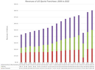
    To value a sports franchise as a business, it is worth examining how the revenues for franchises have evolved over time. Until the last 50 years, almost all of the revenues for sports franchises came from gate receipts collected from fans coming in to watch games, and the food and merchandise that these fans bought, usually at the games they attended. With television entering the picture, and streaming augmenting it, the portion of revenues that sports franchises get from media has become a larger and larger slice of the pie, as can be seen in the graph below, where we look at gate receipts, media revenue and other (merchandizing and sponsorship) revenues for all US sports franchises between 2006 and 2022:

As you can see, the overall revenues for sports franchises has grown between 2006 and 2022, with 2020 being the COVID outlier, but much of that growth has come from the media slice of revenues, as gate receipts have flatlined. This is clearly not just a US phenomenon, and you are seeing the same process play out in Europe (with soccer the big beneficiary) and in India (with cricket the winner). 

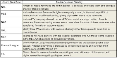
    To value a sports franchise, you not only have to consider how much of a draw the team is at the stadium, but how much revenues the team gets from its media contracts, as well as merchandising and sponsorship revenues. While the gate receipts and merchandising revenues are significant, they are relatively easy to forecast, given history and ticket sales. Media revenues, though, are tricky, since they are determined partly by the size of the media market that the team operates in, and partly by how the sports franchise that the team belongs to shares its media revenues. In the US, for example, baseball teams get a significant portion of their broadcasting revenues from local TV rights, and as a consequence, teams in the biggest media markets (Yankees and Mets in New York, Dodgers in Los Angeles) have higher revenues than teams in smaller media market (Mariners in Seattle). In contrast, the media revenues for football (NFL) are mostly national, and those revenues are equally divided across the teams, resulting in more equitable media revenues across NFL teams. That difference explains why the divergence between the highest and lowest priced teams is greater in baseball than the NFL.  The table below provides a comparison of how media revenues are shared across teams, by franchise:

While all of the franchises pay lip service to the need for balance, with large media-market teams subsidizing small media-market teams, there is wide variation across franchises in how they follow through on fixing that imbalance. Only the NFL has a strong enough system in place to create full balance, and that is partly because of the fact that almost all of its broadcasting revenues are national (rather than local) and partly because it is a league with a strong commissioner.

    While revenues have risen, aided by richer broadcasting contracts, sports franchises have been faced with rising player costs; in almost every major sports franchise in the United States, player expenses account to 50% of revenues, or more, and they have risen over time. Once the other expenses associated with a team are netted out, the operating profits at sports franchises are, for the most part, moderate.  Looking across sports franchises, you can see that the cumulated revenue and operating income numbers, in conjunction with the collective pricing of teams (as estimated by Forbes) in the most recent year:

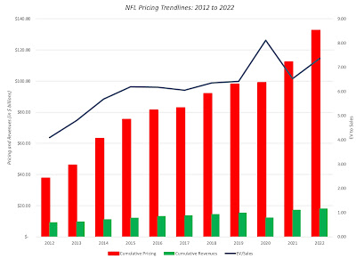
While team financials tend to be opaque, Forbes estimated that the NFL, the richest sports franchise in the world, generated about $4.7 billion in operating profit on revenues of approximately $16 billion, in 2022. The NBA is the next-most profitable franchise, whereas baseball collectively struggles to make money. More to the point, if you use the Forbes pricing estimates for teams, note that four of the seven franchises (NFL, NBA, MLS and IPL) trade at 8-10 times revenues and at high multiples of operating income. It is true that there are tech companies in the market that trade at similar multiples, but those companies have extraordinary growth potential ahead of them and new markets to conquer. Even if you believe that media rights will continue to the the goose that lays the golden eggs for sports franchises, it is difficult to see how you justify these pricing multiples. To show that the disconnect between what buyers are paying for franchises, and what they are getting back in return, has been growing over time, I look at the pricing of NFL teams over time, relative to revenues at these teams (which include the richer media contracts) from 2012 to 2022:

Over the last decade, you can see that the pricing of NFL teams has risen from just over four times revenues in 2012 to more than seven times revenues in 2022. In short, NFL franchise prices are rising at rates that cannot be explained by revenue growth, richer media contracts notwithstanding, or higher profitability.

    If you want to see how intrinsic valuation would work at a sports franchise, you are welcome to check out my intrinsic valuation of the Los Angeles Clippers, when Steve Ballmer offered $2 billion for that franchise in 2014. Looking at four scenarios, ranging from an extrapolation of the Clipper's 2012 financials to a best case scenario, where I modeled out a much larger media revenue stream, I got the following:

Download spreadsheet

I used the same framework to value the Washington Commanders today, and my values range from $2.5 billion, with current profitability, $2.7 billion, if you give them the median operating margin of an NFL team and a value of $4.5 billion, if you give them Dallas Cowboy level margins (the highest in the NFL). In short, getting to the $6.05 billion pricing with an intrinsic valuation is beyond reach.

2. A new breed of owners

    At the start of this section, I mentioned the Rooneys buying the Pittsburg Steelers in 1932 for $2,500, and they continue to own the Steelers. While it is conceivable that they think of the Steelers as a business they own that has to continue to deliver earnings for them, much of the rest of the NFL has seen a changing of the guard, with new owners replacing the older holdouts. Many of these new owners are already wealthy, with their wealth accumulated in a different setting (real estate, private  equity, venture capital), when they buy professional sports teams, and from the outset, it seems clear that they are less interested in turning a profit , and more in playing the role of team owner. To illustrate, I focus on the NBA, where there has been much turnover in the ownership ranks, with close to two-thirds of the teams acquiring new owners in the last two decades:

Source

As you browse this list, you will note that while many of the owners are billionaires, not counting their NBA team ownership, there are a few owners, towards the bottom of the list, whose wealth is primarily in their team ownership.  Looking for trends, the more recent a sports franchise transaction, the more likely it is that the buyer is not just wealthy, but immensely so, and this pattern is playing out across the world.

    So, why would these wealthy, and presumably financially savvy, individuals put their money into sports teams? In keeping with the saying that a picture is worth a thousand words, take a look at this picture of Steve Ballmer on the sidelines of a Clippers game:

To my untrained eye, it seems to me that the Clippers are not just another investment in Ballmer's portfolio. In 2014, at the end of my post on the Clippers, and after attempting in every conceivable way to find a financial justification why Ballmer would pay $2 billion for an NBA team that was a distant second to the other NBA team that played in the same city, I threw up my hands and concluded that Ballmer was buying a toy. By my estimated, it was an expensive toy that I estimated to cost about a billion (my estimate of the difference between the price he paid and my estimated value), but one that he could well afford, given his wealth.

    In many ways, sports franchises are the ultimate trophy assets, since they are scarce and owning them not only allows you to live out your childhood dreams, but also gives you a chance to indulge your friends and family, with front-row seats and player introductions. In fact, it also explains the entry of sovereign wealth funds, especially from the Middle East, into the ownership ranks, especially in the Premier League. If you couple this reality with the fact that winner-take-all economies of the twenty-first century deliver more billionaires in our midst, you can see why there is no imminent correction on the horizon for sports franchise pricing. As long as the number of billionaires exceeds the number of sports franchises on the face of the earth, you should expect to see fewer and fewer owners like the Rooneys and more and more like the Steves (Cohen and Ballmer).

Consequences of Trophy Asset Status

    If you are a sports fan, you may be wondering why any of this matters to you, since you are not a billionaire and are not planning to buy any teams, either as businesses or as trophy assts. I think that you should care because the trophy asset phenomenon is already reshaping how teams are structured, sports get played and perhaps what your favorite team will look like next year, when it takes the field. 

1. For Owners: For the owners of franchises that are not members of the billionaire club, there will be pressure to cash out, and the key to getting a lucrative offer is to increase the team's attraction to potential buyers, as toys. Adding a high-profile player, even one who is approaching the end of his or her playing life, can add to the attraction of a sports team, as a trophy, even as it reduces its quality on the field, as is moving to a city that a potential buyer may view as a better setting for their expensive toy (Oakland A's and San Diego Clipper or Charger fans, take note!). For billionaire owners of franchises, the reactions to owning an expensive toy that does not perform as expected, can range from impatience with managers and players, to trades driven by impulse rather than sports sense. 
2. For Players: As sports franchises become trophy assets, players become the jewels that add dazzle to these trophies. Not surprisingly, the superstars of every sport will be prized even more than they used to be, not just for what they can do on the field, but for what they can do for an owner’s bragging right. The recent billion dollar bid for Mbappe and the upcoming bidding war for Shohei Ohtani make sense from this perspective, and you should expect to see more mind-glowingly large player contracts in the future. To the extent that a player's trophy appeal is as much a function of that player's social media presence and following, as it is of performance  on the field, you should expect to see sports players aspire for celebrity status.
3. For Fans: If you are the fan of a sports franchise that is owned by someone to whom money is no object, you will have much to celebrate, as your team chases down and signs the biggest names in the sport. As a negative, if your team owner tires of their trophy asset, you may be stuck with the consequences of benign (or not so benign) neglect. If on the other hand, you happen to be a fan of the team that continues to be owned by an old-guard owner, intent on running the team as a business, you will find yourself frustrated as homegrown stars get signed by other teams. The old divide of rich teams/poor teams that was based on unequal media markets or stadium sizes will be replaced with a new divide between rich team owners and poorer team owners, where the latter still have to make their teams work as businesses, whereas the former do not.

In sum, if your concern has been that sports has become too business-like and driven by data, the entry of owners who are less interested in the business of sports and more interested in acquiring trophies may very well change the game, but at a cost, where sports becomes entertainment, where players and teams chase social media status, and what happens on the field itself becomes secondary to what happens off the pitch.

YouTube Video

Data

1. Professional Sports Data (Pricing)

Spreadsheets

1. Valuation of the Clippers in 2014
2. Valuation of Washington Commanders in 2023

In Search of Safe Havens: The Trust Deficit and Risk-free Investments!

In every introductory finance class, you begin with the notion of a risk-free investment, and the rate on that investment becomes the base on which you build, to get to expected returns on risky assets and investments. In fact, the standard practice that most analysts and investors follow to estimate the risk free rate is to use the government bond rate, with the only variants being whether they use a short term or a long term rate. I took this estimation process for granted until 2008, when during that crisis, I woke up to the realization that no matter what the text books say about risk-free investments, there are times when finding an investment with a guaranteed return can become an impossible task. In the aftermath of that crisis, I wrote a series of what I called my nightmare papers, starting with one titled, "What if nothing is risk free?", where I looked at the possibility that we live in a world where nothing is truly risk free. I was reminded of that paper a few weeks ago, when Fitch downgraded the US, from AAA to AA+, a relatively minor shift, but one with significant psychological consequences for investors in the largest economy in the world, whose currency still dominates global transactions. After the rating downgrade, my mailbox was inundated with questions of what this action meant for investing, in general, and for corporate finance and valuation practice, in particular, and this post is my attempt to answer them all with one post.

Risk Free Investments: Definition, Role and Measures

    The place to start a discussion of risk-free rates is by answering the question of what you need for an investment to be risk-free, following up by seeing why that risk-free rate plays a central role in corporate finance and investing and then looking at the determinants of that risk-free rate.

What is a risk free investment?

    For an investment to be risk-free, you have feel certain about the return you will make on it. With this definition in place, you can already see that to estimate a risk free rate, you need to be specific about your time horizon, as an investor. 

• An investment that is risk free over a six month time period will not be risk free, if you have a ten year time horizon. That is because you have reinvestment risk, i.e., the proceeds from the six-month investment will have to be reinvested back at the prevailing interest rate six months from now, a year from now and so on, until year 10, and those rates are not known at the time you take the first investment.
• By the same token, an investment that delivers a guaranteed return over ten years will not be risk free to an investor with a six month time horizon. With this investment, you face price risk, since even though you know what you will receive as a coupon or cash flow in future periods, since the present value of these cash flows, will change as rates change. During 2022, the US treasury did not default, but an investor in a 10-year US treasury bond would have earned a return of -18% on his or her investment, as bond prices dropped.

For an investment to be risk free then, it has to meet two conditions. The first is that there is no risk that the issuer of the security will default on their contractual commitments. The second is that the investment generates a cash flow only at your specified duration, and with no intermediate cash flows prior to that duration, since those cash flows will then have to be reinvested at future, uncertain rates. For a five-year time horizon, then, you would need the rate on a five-year zero default-free zero coupons bond as your risk-free rate.

    You can also draw a contrast between a nominal risk-free rate, where you are guaranteed a return in nominal terms, but with inflation being uncertain, the returns you are left with after inflation are no longer guaranteed, and a real risk-free rate, where you are guaranteed a return in real terms, with the investment is designed to protect you against volatile inflation. While there is an appeal to using real risk-free rates and returns, we live in a world of nominal returns, making nominal risk-free rates the dominant choice, in most investment analysis.

Why does the risk-free rate matter?

    By itself, a risk-free investment may seem unexceptional, and perhaps even boring, but it is a central component of investing and corporate finance:

1. Asset Allocation: Investors vary on risk aversion, with some more willing to take risk than others. While there are numerous mechanisms that they use to reflect their differences on risk tolerance, the simplest and the most powerful is in their choice on how much to invest in risky assets (stocks, corporate bonds, collectibles etc.) and how much to hold in investments with guaranteed returns over their time horizon (cash, treasury bill and treasury bonds).
2. Expected returns for Risky Investments: The risk-free rate becomes the base on which you build to estimate expected returns on all other investments. For instance, if you read my last post on equity risk premiums, I described the equity risk premium as the additional return you would demand, over and above the risk free rate. As the risk-free rate rises, expected returns on equities will be pushed up, and holding all else constant, stock prices will go down., and the reverse will occur, when risk-free rates drop.
3. Hurdle rates for companies: Using the same reasoning, higher risk-free rates push up the costs of equity and debt for all companies, and by doing so, raise the hurdle rates for new investments. As you increase hurdle rates, new investments will have to earn higher returns to be acceptable, and existing investments can cross from being value-creating (earning more than the hurdle rate) to value-destroying (earning less). 
4. Arbitrage pricing: Arbitrage refers to the possibility that you can create risk-free positions by combining holdings in different securities, and the benchmark used to judge whether these positions are value-creating becomes the risk-free rate. If you do assume that markets will price away this excess profit, you then have the basis for the models that are used to value options and other derivative assets. That is why the risk-free rate becomes an input into option pricing and forward pricing models, and its absence leaves a vacuum.

Determinants

    So, why do risk-free rates vary across time and across currencies? If your answer is the Fed or central banks, you have lost the script, since the rates that central banks set tend to be short-term, and inaccessible, for most investors. In the US, the Fed sets the Fed Funds rate, an overnight intra-bank borrowing rate, but US treasury rates, from the 3-month to 30-year, are set at auctions, and by demand and supply. To understand the fundamentals that determine these rates, put yourself in the shoes of a buyer of these securities, and consider the following:

1. Inflation: If you expect inflation to be 3% in the next year, it makes little sense to buy a bond, even if it is default free, that offers only 2%. As expected inflation rises, you should expect risk-free rates to rise, with or without central bank actions. 
2. Real Interest Rate: When you buy a note or a bond, you are giving up current consumption for future consumption, and it is fitting that you earn a return for this sacrifice. This is a real risk-free rate, and in the aggregate, it will be determined by the supply of savings in an economy and the demand for those savings from businesses and individuals making real investments. Put simply, economies with a surplus of growth investments, i.e., with more real growth, should see higher real interest rates, in steady state, than stagnant or declining economies.

The recognition of these fundamentals is what gives rise to the Fisher equation for interest rates or the risk free rate:

    Nominal Risk-free Rate = (1 + Expected Inflation) (1+ Real Interest Rate) -1 (or)

                                            =  Expected Inflation + Expected Real Interest Rate (as an approximation)

If you are wondering where central banks enter this equation, they can do so in three ways. The first is that central banking actions can affect expected inflation, at least in the long term, with more money-printing leading to higher inflation. The second is central banking actions can, at least at the margin, push rates above their fundamentals (expected inflation and real interest rates), by tightening monetary policy, and below their fundamentals by easing monetary policy. Since this is often achieved by raising or lowering the very short term rates set by the central bank, the central banking effect is likely to be greater at the shorter duration risk-free rates. The third is that central banks, by tightening or easing monetary policy, may affect real growth in the near term, and by doing so, affect real rates. 

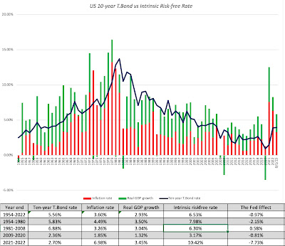
    Having been fed the mythology that the Fed (or another central bank) set interest rates by investors and the media, you may be unconvinced, but there is no better way to show the emptiness of "the Fed did it" argument than to plot out the US treasury bond rate each year against a crude version of the fundamental risk-free rate, computed by adding the actual inflation in a year to the real GDP growth rate that year:

As you can see, the primary reasons why we saw historically low rates in the 2008-2021 time period was a combination of very low inflation and anemic real growth, and the main reason that we have seen rates rise in 2022 and 2023 is rising inflation. It is true that nominal rates follow a smoother path than the intrinsic risk free rates, but that is to be expected since the ten-year rates represent expected values for inflation and real growth over the next decade, whereas my estimates of the intrinsic rates represent one-year numbers. Thus, while inflation jumped in 2021 and 2022 to 6.98%, and investors are expecting higher inflation in the future, they are not expecting inflation to stay at those levels for the next decade.    

Risk Free Rate: Measurement

    Now that we have established what a risk-free rate is, why it matters and its determinants, let us look at how best to measure that risk-free rate. We will begin by looking at the standard practice of using government bond rates as riskfree rates, and why it collides with reality, move on to examine why governments default and end with an assessment of how to adjust government bond rates for that default risk.

Government Bond Rates as Risk Free

    I took my first finance class a long, long time ago, and during the risk-free rate discussion, which lasted all of 90 seconds, I was told to use the US treasury rate as a risk-free rate. Not only was this an indication of how dollar-centric much of finance education used to be, but also of how much faith there was that the US treasury was default-free. Since then, as finance has globalized, that lesson has been carried, almost unchanged, into other currencies, where we are now being taught to use government bond rates in those currencies as risk-free rates. While that is convenient, it is worth emphasizing two implicit assumptions that underlie why government bond rates are viewed as risk-free:

1. Control of the printing presses: If you have heard the rationale for government bond rates as risk-free rates, here is how it usually goes. A government, when it borrows or issues bonds in its local currency, preserves the option to print more money, when that debt comes due, and thus should never default. This assumption breaks down, of course, when countries share a common currency, as is the case with the dozen or more European countries that all use the Euro as their domestic currency, and none of them has the power to print currency at will. 
2. Trust in government: Governments that default, especially on their domestic currency borrowings, are sending a signal that they cannot be trusted on their obligations, and the implicit assumption is that no government that has a choice would ever send that signal. (Governments send the same signal when they default on their foreign currency debt/bonds, but they can at least point to circumstances out of their control for doing so.)

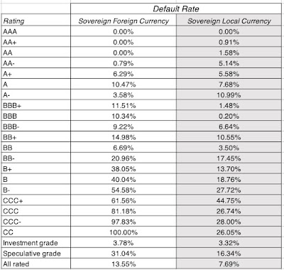
The problem with these assumptions is that they are at war with the data. As we noted in our country risk discussion, governments do default on their local currency borrowings and bonds, albeit at a lower rate than they do on their foreign currency obligations. 

If you are wondering why a government that has a choice of not defaulting would choose to default, it is worth remembering that printing more money to pay off local currency debt has a cost of its own, since it debases the currency, pushing up inflation. Inflation, especially when it becomes stratospheric, causes investors and consumers to lose trust in the currency, and given a choice between default and debasement, many governments choose the latter.

    Once you open the door to the possibility of sovereign default in a local currency, it stands to reason that a government bond rate in the local currency may not always yield a risk-free rate for that currency. It is also worth noting that until 2008, investors had that door firmly shut for some currencies, believing that some governments were so trustworthy that they would not even consider default. Thus, the notion that the US or UK governments would default on their debt would have been unthinkable, but the 2008 crisis, in addition to the financial damage it created, also opened up a trust deficit, which has made the unthinkable a reality. In fact, you would be hard pressed to find any government that is trusted the way it was prior to this crisis, and that loss of trust also implies that the clock is ticking towards expiration, for the "government bonds are risk free" argument.

When and Why Governments Default

    Now that we have established that governments can default, let’s look at why they default. The most obvious reason is economic, where a crisis and collapse in government revenues, from taxes and other sources, causes a government to be unable meet its obligations. The likelihood of this happening should be affected by the following factors:

1. Concentrated versus Diversified Economy: A government's capacity to cover its debt obligations is a function of the revenues it generates, and those revenues are likely to be more volatile in a country that gets its revenues from a single industry or commodity than it is in a country with a more diverse economy. One measure of economic concentration is the percent of GDP that comes from commodity exports, and the picture below provides that statistic, by country:

   

   Source: UNCTAD

   
   
   As you can see, much of Africa, Latin America, the Middle East and Asia are commodity dependent, effectively making them more exposed to default, with a downturn in commodity prices.
2. Degree of Indebtedness: As with companies, countries that borrow too much are more exposed to default risk than countries that borrow less. That said, the question of what to scale borrowing to is an open question. One widely-used measure of country indebtedness is the total debt owed by the country, as a percent of its GDP. Based on that statistic, the most indebted countries are listed below:
   
   As you can see, this table contains a mix of countries, with some (Venezuela, Greece and El Salvador) at high risk of default and others (Japan, US, UK, Canada and France) viewed as being at low risk of default. 
3. Tax Efficiency: It is worth remembering that governments do not cover debt obligations with gross domestic product or country wealth, but with their revenues, which come primarily from collecting taxes. Holding all else constant, governments with more efficient tax systems, where most taxpayers comply and pay their share, are less likely to default than governments with more porous tax systems, where tax evasion is more the rule than the exception, and corruption puts revenues into the hands of private players rather than the government.

There is a second force at play, in sovereign defaults. Ultimately, a government that chooses to default is making a political choice, as much as it is an economic one. When politics is functional, and parties across the spectrum share in the belief that default should be a last resort, with significant economic costs, there will be shared incentive in avoiding default. However, when politics becomes dysfunctional, and default is perceived as partisan, with one side of the political divide perceived as losing more from default than the other, governments may default even though they have the resources to cover their obligations.

    As a lender to a government, you may not care about why a government defaults, but economic defaults generally represent more intractable problems than defaults caused by political dysfunction, which tend to be solved once the partisan pounds of flesh are extracted. In my view, the ratings downgrades of the US government fall into the latter category, since they are triggered by a uniquely US phenomenon, which is a debt limit that has to be reset each time the total debt of the US approaches that value. Since that reset has to be approved by the legislature, it becomes a mechanism for political standoffs, especially when there is a split in executive and legislative power. In fact, the first downgrade of the US occurred more than a decade ago, when S&P lowered its sovereign rating for the US from AAA to AA+ in 2011, after a debt-limit standoff at the time. The Fitch downgrade of the US, this year, was triggered by a stand-off between the administration and Congress a few months ago on the debt-limit, and one that may be revisited in a few weeks again. 

Measuring Government Default Risk

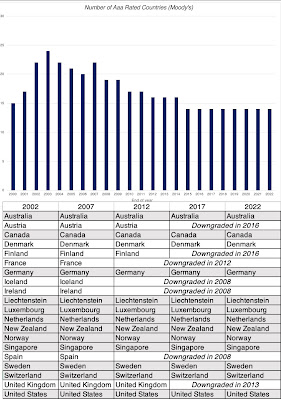
    With that lead-in on sovereign default risk, let us look at how sovereign default risk gets measured, again with the US as the focus. The first and most widely used measure of default risk is sovereign ratings, where ratings agencies rate countries, just as they do companies, with a rating scale that goes from AAA (Aaa) down to D(default). Fitch, Moody's and S&P all provide sovereign ratings for countries, with separate ratings for foreign currency and local currency debt. With sovereign ratings, the implicit assumption is that AAA (Aaa) rated countries have negligible or no default risk, and the ratings agencies back this up with the statistic that no AAA rated country has ever defaulted on its debt within 15 years of getting a AAA rating. That said, the number of AAA (Aaa) rated countries has dropped over time, and there are only nine countries left that have the top rating from all three ratings agencies: Germany, Denmark, Netherlands, Sweden, Norway, Switzerland, Luxembourg, Singapore and Australia. Canada is rated AAA by two of the ratings agencies, and after the Fitch downgrade, the US is rated Aaa only by Moody's, whereas the UK is AAA rated only by S&P.

   In a reflection of the times, there have been two developments. The first is that the number of countries with the highest rating has dropped over time, as can be seen in the graph below of countries with Aaa ratings from Moody's: 

Second, even the ratings agencies have become less decisive about what a AAA sovereign rating implies for default risk, especially after the 2008 crisis, when S&P announced that not all AAA countries were equal, in terms of default risk, thus admitting that each ratings class included variations in default risk. 

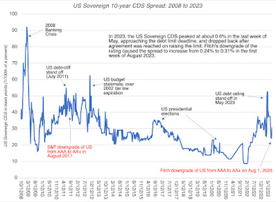
    If you recognize that default risk falls on a continuum, rather than in the discrete classes that ratings assign, the sovereign CDS market gives you not only more nuanced estimates of default risk, but ones that are reflect, on an updated basis, what investors think about a country's default risk. The graph below contains the sovereign CDS spreads for the US going back to 2008, and reflect the market's reactions to events (including the 2011 and 2023 debt-limit standoffs) over time:

As you can see, the debt-limit and tax law standoffs created spikes in 2011 and 2012, and, to a lesser extent, in early 2023, and that these spikes preceded the ratings changes, and were not caused by them, and that the market very quickly recovered from them. In fact, the Fitch ratings downgrade has barely registered on the US CDS spread, in the market, indicating that investors are neither surprised nor spooked by the ratings downgrades (so far). 

Dealing with Government Default Risk

     No matter what you think about the Fitch downgrade of US government debt, the big-picture perspective is that we are closer to the scenario where no entity is viewed as default-free than we were fifteen years ago, and it may be only a matter of time before we have to retire the notion that government bonds are default-free entirely. The questions for investors and analysts, if this occurs, becomes practical ones, including how best to estimate risk-free rates in currencies, when governments have default risk, and what the consequences are for equity risk premiums and default spreads.

1. Clean up government bond rate

    Consider the two requirements that have to be met for a local-currency government bond rate to be used as a risk-free rate in that currency. The first is that the government bond has to be widely traded, making the interest rate on the bond a rate set by demand and supply in the market, rather than government edict. The second is that the government be perceived as default-free. The Swiss 10-year government bond rate, in July 2023, of 1.02% meets both criteria, making it the risk-free rate in Swiss Francs. Using a similar rationale, the German 10-year bund rate (in Euros) of 2.47% becomes the risk-free rate in Euros. With the British pound, if you stay with the Moody's ratings, things get trickier. The government bond rate of 4.42% is no longer risk-free, because it has default risk embedded in it. To clean up that default risk, we estimated a default spread of 0.64%, based upon UK's rating of Aa3, and netted this spread out from the government bond rate:

Risk-free Rate in British Pounds     

= Government Bond Rate in Pounds - Default Spread for UK = 4.42% - 0.64% = 3.78%

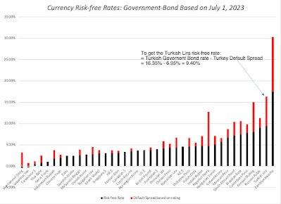
Extending this approach to all currencies, where there is a government bond rate present, we get the riskfree rates in about 30 currencies:

Since the US still preserves a bond rating of Aaa (for the moment), with Moody's, the US treasury rate of 3.77% on July 1, 2023, was used as the riskfree rate in US dollars. 

    As you look at these rates, especially in some emerging market currencies, you should be cautious about the numbers you get, especially since the liquidity is light or non-existent in government bonds in these markets. Thus, it is possible that the Vietnamese Dong has the lowest risk-free rate in the world in mid-2023, among all currencies, or it may reflect distortions in the Vietnamese government bond.   One way to check these riskier rates for reasonableness is to extend on the insight that the key driver of the risk free rate is inflation, and that in a world where capital moves to equalize real returns, the differences in risk-free rates across currencies come from differential inflation In my post on country risk, In fact, as I argued in my post on country risk, you can convert a riskfree rate in any currency into a risk-free rate in another currency by adjusting for the differential inflation between the currencies: 

Thus, using the IMF's forecasted inflation rates for the US (3%) and Vietnam (5.08%), in conjunction with the US dollar risk-free rate of 3.77% on July 1, 2023, yields a Vietnamese Dong risk-free rate of 5.87% (or 5.85% with the approximation).

    If you believe that S&P and Fitch are right on their default risk assessments for the US, and that it should get a rating lower than Aaa (say Aa1), from Moody's, the path to getting a US risk-free rate has an added step. You have to net out the default spread for the US treasury bond rate to get to a risk-free rate:

Riskfree Rate in US dollars = US Treasury Bond Rate - Default spread on US T.Bond

Using the sovereign CDS market's estimate of 0.30% in August 2023, for instance, when the US treasury bond rate hit 4.10%, would have yielded a risk-free rate of 3.80% for the US dollar.

2. Risk Premia

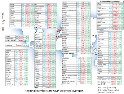
    If you focus just on risk-free rates, you may find it counter intuitive that an increase in default risk for a country lowers the risk free rate in its currency, but looking at the big picture should explain why it is necessary. An increase in sovereign default risk is usually triggered by events that also increase risk premia in markets, pushing up government bond rates, equity risk premiums and default spreads. In fact, if you go back to my post on country risk, it becomes the key driver of the additional risk premiums that you demand in countries:

You will notice that in my July 2023 update, I used the implied equity risk premium for the US of 5.00% as my estimate of a premium for a mature market, and assumed that any country with a Aaa  rating (from Moody's) would have the same premium. 

    Since Moody's remains the lone holdout on downgrading the US, I would use the same approach today, but assuming that Moody's downgrades the US from Aaa to Aa1, the approach will have to be modified. The implied equity risk premium for the US will still be my starting point, but countries with Aaa ratings will then be assigned equity risk premiums lower than the US, and that lower equity risk premium will become the mature market premium, to be used to get equity risk premiums for the rest of the world. Using the sovereign CDS spread of 0.30% as the basis, just for illustration, the mature market premium would drop from 5.00%, in my July 2023 update, to 4.58% (5.00% -1.42*.30%).

When safe havens become scarce...

    During crises, investors seeks out safety, but that pre-supposes that there is a safe place to put your money, where you know what you will make with certainty. The Fitch downgrade of the US, by itself, is not a market-shaking event, but in conjunction with a minus 18% return on the ten-year US treasury bond in 2022, these events undercut the notion that there is a safe haven for investors. When there is no safe haven, market corrections when they happen will not follow predictable patterns. Historically, when stock prices have plunged, investors have sought out US treasuries, pushing down yields and prices. But what if government securities are viewed as risky? Is it any surprise that the loss of trust in governments that has undercut the perception that they are default-free has also given rise to a host of other investment options, each claiming to be the next safe haven. While my skepticism about crypto currencies and NFTs is well documented, a portion of their rise over the last 15 years has been driven by the erosion of trust in institutions. 

Conclusion

    I started this post by noting that we pay little attention to risk-free rates in theory and in practice, taking it as a given that it is easy to estimate. As you can see from this post, that casual acceptance of what comprises a risk-free investment can be a recipe for disaster. In closing, here are a few general propositions about risk-free rates that are worth keeping in mind:

1. Risk-free rates go with currencies, not countries or governments: You estimate a risk-free rate in Euros or dollars, not one for the Euro-zone or the United States. Thus, if you choose to analyze a Brazilian company in US dollars, the risk-free rate you should use is the US dollar risk free rate, not the rate on Brazilian US-dollar denominated bond. It follows, therefore, that the notion of a global risk-free rate, touted by some, is fantasy, and using the lowest government bond rate, ignoring currencies, as an estimate of this rate, is nonsensical.
2. Investment returns should be currency-explicit and time-specific: Would you be okay with a 12% return on a stock, in the long term? That question is unanswerable, until you specify the currency in which you are denominating returns, and the time you are making the assessment. An investment that earns 12%, in Zambian Kwacha, may be making less than the risk-free rate in Kwachas, but one that earns that same return in Swiss Francs should be a slam-dunk as an investment. In the same vein, an investment that earns 12% in US dollars in 2023 may well pass muster as a good investment, but an investment that earned 12% in US dollars in 1980 would not (since the US treasury bond rate would have yielded more than 10% at the time).
3. Currencies are measurement mechanisms, not value-enhancer or destroyers: A good financial analysis or valuation should be currency-invariant, with whatever conclusion you draw when you do your analysis in one currency carrying over into the same analysis, done in different currencies. Thus, switching from a currency with a high risk-free rate to one with a much lower risk-free rate will lower your discount rate, but the inflation differential that causes this to happen will also lower your cash flows by a proportional amount, leaving your value unchanged.
4. No one (including central banks) cannot fight fundamentals: Central banks and governments that think that they have the power to raise or lower interest rates by edict, and the investors who invest on that basis, are being delusional. While they can nudge rates at the margin, they cannot fight fundamentals (inflation and real growth), and when they do, the fundamentals will win.

YouTube Video

The Price of Risk: With Equity Risk Premiums, Caveat Emptor!

    If you have been reading my posts, you know that I have an obsession with equity risk premiums, which I believe lie at the center of almost every substantive debate in markets and investing. As part of that obsession, since September 2008, I have estimated an equity risk premium for the S&P 500 at the start of each month, and not only used that premium, when valuing companies during that month, but shared my estimate on my webpage and on social media. In my last post, on country risk premiums, I used the equity risk premium of 5.00% that I estimated for the US at the start of July 2023, for the S&P 500. That said, I don't blame you, if are confused not only about how I estimate this premium, but what it measures. In fact, an article in MarketWatch earlier this year referred to the equity risk premium as an esoteric concept, a phrasing that suggested that it had little relevance to the average investor. Adding to the confusion  are the proliferation of very different numbers that you may have seen attached to the current equity risk premium, each usually quoting an expert in the field, but providing little context. Just in the last few weeks, I have seen a Wall Street Journal article put the equity risk premium at 1.1%, a Reuters report put it at 2.2%, and a bearish (and widely followed) money manager estimate the equity risk premium to be negative. How, you may ask, can equity risk premiums be that divergent, and does that imply that anything goes? In this post, I will not try to argue that my estimate is better than others, since that would be hubris, but instead focus on explaining why these ERP differences exist, and let you make your own judgment on which one you should use in your investing decisions.

ERP: Definition and Determinants

    The place to start this discussion is with an explanation of what an equity risk premium is, the determinants of that number and why it matters for investors. I will try to steer away from models and economic jargon in this section, simply because they do little to advance understanding and much to muddy the waters.

What is it?

    Investors are risk averse, at least in the aggregate, and while that risk aversion can wax and wane, they need at least the expectation of a higher return to be induced to invest in riskier investments. In short, the expected return on a risky investment can be constructed as the sum of the returns you can expect on a guaranteed investment, i.e.,  a riskfree rate, and a risk premium, which will scale up as risk increases. 

Expected Return = Risk free Rate + Risk Premium

Note that this proposition holds even if you believe that there is nothing out there that is truly risk free, which is the case when you worry about governments defaulting, though it does imply that you have cleaning up to do to get to a riskfree rate. Note also that expectations do not always pan out, and the actual returns on a risky investment can be much lower than the risk free rate, and sometimes sharply negative.

    The risk premium that you demand has different names in different markets. In the corporate bond market, it is a default spread, an augmentation to the interest rate that you demand on a bond with more default risk. In the real estate market, it is embedded in a capitalization rate, an expected return used by real estate investors to convert the income on a real estate property into a value for that property. In the equity market, it is the equity risk premium, the price of risk for investing in equities as a class.

As you can see, every asset class has a risk premium, and while those risk premiums are set by investors within each asset class, these premiums tend to move together much of the time.

Determinants

    Since the equity risk premium is a price for risk, set by demand and supply, it stands to reason that it is driven not only by economic fundamentals, but also by market mood. Equities represent the residual claim on the businesses in an economy, and it should come as no surprise that the fundamentals that determine it span the spectrum:

My equity risk premium paper

Even a cursory examination of these fundamentals should lead you to conclude that not only will equity risk premiums vary across markets, providing an underpinning for the divergence in country risk premiums in my last post, but should also vary across time, since the fundamentals themselves change over time. 

    Market prices are also driven by mood and momentum, and not surprisingly, equity risk premiums can change, as these moods shift. In particular, equity risk premiums can become too low (too high) if investors are excessively upbeat (depressed) about the future, and thus become the ultimate receptacles for market hope and fear. In fact, one symptom of a market bubble is an equity risk premium that becomes so low that it is disconnected from fundamentals, setting up for an inevitable collision with reality and a market correction.

Why it matters

    If you are a trader, an investor or a market-timer, and you are wondering why you should care about this discussion, it is worth recognizing that the equity risk premium is a central component of what you do, even if you have never explicitly estimated or used it.

1. Market Timing: When you time markets, you are making a judgment on how an entire asset class (equities, bonds, real estate) is priced, and reallocating your money accordingly. In particular, if you believe that stocks are over priced, you will either have less of your portfolio invested in equities or, if you are aggressive, sell short on equities. Any statement about market pricing can be rephrased as a statement about equity risk premiums; if you believe that the equity risk premium, as priced in by the market, has become too low (relative to what you believe is justified, given history and fundamentals), you are arguing that stocks are over priced (and due for a correction). Conversely, if you believe that the equity risk premium has become too high, relative again to what you think is a reasonable value, you are contending that stocks are cheap, in the aggregate.  
2. Stock Picker: When you invest in an individual stock, you are doing so because you believe that stock is trading at a price that is lower than your estimate of its value. However, to make this judgment, you have to assess value in the first place, and while we can debate growth potential and profitability, the equity risk premium becomes an input into the process, determining what you should earn as an expected return on a stock. Put simply, if you are using an equity risk premium in your company valuation that is much lower (higher) than the market-set equity risk premium, you are biasing yourself to find the company to be under (over) valued. A market-neutral valuation of a company, i.e., a valuation of the company given where the market is today, requires you to at least to try to estimate a premium that is close to what the market is pricing into equities.
3. Corporate Finance: The role of the equity risk premium in determining the expected return on a stock makes it a key input in corporate finance, as well, because that expected return becomes the company's cost of equity. That cost of equity is then embedded in a cost of capital, and as equity risk premiums rise, all companies will see their costs of capital rise. In a post from the start of this year, I noted how the surge in equity risk premiums in 2022, combined with rising treasury bond rates, caused the cost of capital to increase dramatically during the course of the year.

Put simply, the equity risk premiums that we estimate for markets have consequences for investors and businesses, and in the next section, I will look at ways of estimating it.

Measurement

    If the equity risk premium is a market-set number for the price of risk in equity markets, how do we go about estimating it? Unlike the bond market, where interest rates on bonds can be used to back out default spreads, equity investors are not explicit about what they are demanding as expected returns when they buy stocks. As a consequence, a range of approaches have been used to estimate the equity risk premium, and in this section, I will look at the pluses and minuses of each approach.

1. Historical Risk Premium

    While we cannot explicitly observe what investors are demanding as equity risk premiums, we can observe what they have earned historically, investing in stocks instead of something risk free (or close). In the US, that data is available for long periods, with the most widely used datasets going back to the 1920s, and that data has been sliced and diced to the point of diminishing returns. At the start of every year, I update the data to bring in the most recent year's returns on stocks, treasury bonds and treasury bills, and the start of 2023 included one of the most jarring updates in my memory:

Spreadsheet with historical data

It was an unusual year, not just because stocks were down significantly, but also because the ten-year treasury bond, a much touted safe investment, lost 18% of its value. Relative to treasury bills, stocks delivered a negative risk premium in 2022 (-20%), but it would be nonsensical to extrapolate from a single year of data. In fact, even if you stretch the time periods out to ten, fifty or close to hundred years, you will notice that your estimates of expected returns come with significant error (as can be seen in the standard errors). 

    In much of valuation, especially in the appraisal community, historical risk premiums remain the prevalent standard  for measuring equity risk premiums, and there are a few reasons. 

• Perhaps, the fact that you can compute averages precisely gets translated into the delusion that these averages are facts, when, in fact, they are not just estimates, but very noisy ones. For instance, even if you use the entire 94-year time period (from 1928-2022), your estimate for the equity risk premium for stocks over ten-year treasury bonds is that it falls somewhere between 2.34% to 10.94%, with 95% confidence (6.64% ± 2* 2.15%). 
• It is also true that the menu of choices that you have for historical equity risk premiums, from a low of 4.12% to a high of 13.08%, depending on then time period you look at, and what you use as a riskfree rate, gives analysts a chance to let their biases play out. After all, if your job is to come up with a low value, all you have to do is latch on to a high number in this table, claim that it is a historical risk premium and deliver on your promise. 

   When using historical equity risk premiums, you are assuming mean reversion, i.e., that returns revert  to historic norms over time, though, as you can see, those norms can be different, using different time periods. You are also assuming that the economic and market structure has not changed significantly over the estimation period, i.e., that the fundamentals that determine the risk premium have remained stable. For much of the twentieth century, historical equity risk premiums worked well as risk premium predictors in the United States, precisely because these assumptions held up. With China's rise, increased globalization and the crisis of 2008 as precipitating factors, I would argue that the case for using historical risk premiums has become much weaker.

2. Historical Returns-Based Forecasts

    The second approach to using historical returns to estimate equity risk premiums starts with the same data as the first approach, but rather than just use the averages to make the estimates, it looks for time series patterns in historical returns that can be used to forecast expected returns. Put simply, this approach brings into the estimate the correlation across time in returns:

If the correlations across time in stock returns were zero, this approach would yield results similar to just using the averages (historical risk premiums), but it they are not, it will lead to different predictions. Looking at historical returns, the correlations start off close to zero for one-year returns but they do become slightly more negative as you lengthen your time periods; the correlation in returns over 5-year time periods is -0.15, but it is not statistically significant. However, with 10-year time horizon, even that mild correlation disappears. In short, while it may be possible to coax a predictive model using only historical stock returns, that model is unlikely to yield much in actionable predictions. There are sub-periods where the correlation is higher, but I remain skeptical of any ERP prediction model built around just the time series of stock returns.

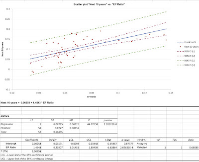
    In an extension of this approach, you could bring in a measure of the cheapness of stocks (PE ratios or earnings yields are the most common ones) into the historical return data and exploit the relationship (if any) between the two. If there is a relationship, positive or negative, between PE ratios and subsequent returns, a regression of returns against PE (or EP) ratios can be used to generate predictions of expected annual returns in the next year, next 5 years or the next decade. The figure below is the scatter plot of earnings to price ratios against stock returns in the subsequent ten years, using data from 1960 to 2022:

A regression using this data yields some of the lowest estimates of the ERP, especially for longer time horizons, because of the elevated levels of PE ratios today. In fact, at the current EP ratio of about 4%, and using the historical statistical link with long-term returns, the estimated expected annual return on stocks, over the next 10 years and based on this regression is:

• Expected Return on Stocks, conditional on EP = .00254 + 1.4543 (.04) = .0607 or 6.07%
• ERP based on EP-based Expected Return = 6.07% - 3.97% = 2.10%

It is worth remembering that the expected return predictions come with error, and the more appropriate use of this regression is to get a range for the expected annual return, which yields predictions ranging from 4% to 8%. Extending the regression back to 1928 increases the R-squared and results in some regressions that yield predicted stock returns that are lower than the treasury-bond rate, i.e., a negative equity risk premium, given the EP ratio today. 

    Note that the results from this regression just reinforce rules of thumb for market timing, based upon PE ratios, where investors are directed to sell (buy) stocks if PE ratios move above (below) a “fair value” band. Since those rules of thumb have yielded questionable results, it pays to be skeptical about these regressions as well, and there are three limitations that those who use it have to keep in mind. 

• First, with the longer time-period predictions, where the predictive power is strongest, the same data is counted multiple times in the regression. Thus, with 5-year returns, you match the EP ratio at the end of 1960 with returns from 1961 to 1965, and then the EP ratio at the end of 1961 with returns from 1962 to 1966, and so on. While this does not imply that you cannot run these regression, it does indicate that the statistical significance (R squared and t statistics) are overstated for the longer time horizons. In addition, the longer your time horizon, the more data you lose. With a 10-year time horizon, for instance, the last year that you can use for predictions is 2012, with the EP ratio in that year matched up to the returns from 2013-2022. 
• Second, as is the case with the first approach (historical risk premiums), you are assuming  that the structural model is stable and that there will be mean reversion. In fact, within this time period (1928 - 2022), the predictive power is far greater between 1928 and 1960 than it is betweeen 196 and 2022.
• Third, while these models tout high R-squared, the number that matters is the standard error of the predictions. Predicting that your annual return will be 6.07% for the next decade with a standard error of 2% yields a range that leaves you, as an investor, in suspended animation, since you face daunting questions about follow through: Does a low expected return on stocks over the next decade mean that you should pull all of your money out of equities? If yes, where should you invest that cash? And when would you get back into equities again?

Proponents of this approach are among the most bearish investors in the market today, but it is worth noting that this approach would have yielded “low return” predictions and kept you out of stocks for much of the last decade. 

3. The Fed Model: Earnings Yield and ERP

    The problem with historical returns approaches is that they are backward-looking, when equity risk premiums should be about what investors expect to earn in the future. To the extent that value is driven by expected future cash flows, you can back out an equity risk premium from current stock prices, if you are willing to make assumptions about earnings growth and cash flows in the future. In the simplest version of this approach, you start with a stable-growth dividend discount model, where the value of equity can be written as the present value of dividends, growing at a constant rate forever:

If you assume that earnings will stagnate at current levels, i.e., no earnings growth, and that companies pay out their entire earnings as dividends (payout ratio = 100%), the cost of equity can be approximated by the earnings to price ratio:

Alternatively, you can assume that there is earnings growth and that companies earn returns on equity equal to their costs of equity, you arrive at the same result:

In short, the earnings to price ratio becomes a rough proxy for what you can expect to earn as a return on stocks, if you are willing to assume no earnings growth or that firms generate no excess returns.

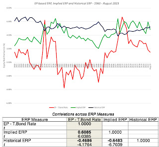
    This is the basis for the widely used Fed model, where the earnings yield is compared to the treasury bond rate, and the equity risk premium is the difference between the two. In the figure below, you can see the equity risk premiums over time that emerge from this comparison, on a quarterly basis, from 1988 to 2023:

Download quarterly data

As you can see, this approach yields some "strange" numbers, with negative equity risk premiums for much of the 1990s, one of the best decades for investing in stocks over the last century. It is true that the equity risk premiums have been much more positive in this century, but that is largely because the treasury bond rate dropped to historic lows, after 2008. As interest rates have risen over the last year and a half,  with stock prices surging over the same period, the equity risk premium based on this approach has dropped, standing at 0.41% at the start of August 2023. Since this is the approach used in the Wall Street Journal article, it explains the ERP being at a two-decade low, but I do find it odd that there is no mention that this approach yielded negative premiums in the 1980s and 1990s. In a variant, the Wall Street Journal article also looks at the difference between the earnings yield and the inflation-protected treasury rate, which yields a higher value for the ERP, of about 3%, but suffers from many of the same issues as the standard approach.

    My problem with the earnings yield approach to estimating equity risk premiums is that the assumptions that you need to make to justify its use are are at war with the data. First, while earnings growth for US stocks has been negative in some years, it has been positive every decade for the last century, and there are no analysts (that I am aware of) expecting it be zero (in nominal terms) in the future. Second, assuming that the return on equity is equal to the cost of equity may be easy on paper, but the actual return on equity for companies in the S&P 500 was 19.73% in 2022, 17.04% over the last decade and has been higher than the cost of equity even in the worst year in this century (9.35% in 2008). If you allow for growth in earnings and excess returns, it is clear that earnings yield will yield too low a value for the ERP, because of these omissions, and will yield negative values in many periods, making it useless as an ERP estimator for valuation.

4. Implied ERP

    I start with the same general model for value that the earnings yield approach does, which is the dividend discount model but change three components

1. Augmented Dividends: It is undeniable that companies around the world, but especially in the US, have shifted from returning cash in the form of dividends to stock buybacks. Since two-thirds of the cash returned in 2022 was in the form of buybacks, ignoring them will lead to understating expected returns and equity risk premiums. Consequently, I add buybacks to dividends to arrive at an augmented measure of cash returned and use that as the base for my forecasts.
2. Allow for near-term growth in Earnings: Since the objective is to estimate what investors are demanding as an expected return, given their expectations of growth, I use analyst estimates of growth in earnings for the index. To get these growth rates, I focus on analysts who estimate aggregated earnings growth the index, rather than aggregating the growth rates estimated by analysts for individual companies, where you risk double counting buybacks (since analyst estimates are often in earnings per share) and bias (since company analysts tend to over estimated growth).
3. Excess Returns and Cashflows: I start my forecasts by assuming that companies will return the same percentage of earnings in cash flows, was they did in the most recent year, but I allow for the option of adjusting that cash return percentage over time, as a function of growth and return on equity (Sustainable cash payout = Growth rate/ Return on Equity). 

The resulting model in its generic form is below:

In August 2023, this model would have yielded an equity risk premium of 4.44% for the S&P 500, using trailing cash flows from the last twelve months as a starting point, estimating aggregate earnings for the companies from analyst estimates, for the next three years, and then scaling that growth down to the risk free rate, as a proxy for nominal growth in the economy, after year 5:

Download implied ERP spreadsheet

To reconcile my estimate of the equity risk premium with the earnings yield approach, you can set the earnings growth rate to zero and the cash payout to 100%, in this model, and you will find that the equity risk premium you get converges on the 0.41% that you get with the earnings yield approach. Adding growth and excess returns to the equation is what brings it up to 4.44%, and I believe that the data is on my side, in this debate. To the critique that my approach requires estimates of earnings growth and excess returns that may be wrong, I agree, but I am willing to wager that whatever mistakes I make on either input will be smaller than the input mistakes made by assuming no growth and no excess returns, as is the case with the earnings yield approach.

Picking an Approach

   I prefer the implied equity risk premium approach that I just described, as the best estimate of ERP,  but that may just reflect my comfort with it, developed over time. Ultimately, the test of which approach is the best one for estimating equity risk premium is not theoretical, but pragmatic, since your estimate of the equity risk premium is used to obtain predictions of returns in subsequent periods. In the figure below, I highlight  three estimates of equity risk premiums - the historical risk premium through the start of that year and the EP-based ERP (EP Ratio minus the T.Bond Rate) and the implied equity risk premiums, at the start of the year:

The historical risk premium is stable, but that stability is a reflection of a having a long tail of historical data that keeps it from changing, even after the worst of years. The implied and EP-based ERP approaches move in the same direction much of the time (as evidenced in the positive correlation between the two estimates), but the latter yields negative values for the equity risk premium in a large number of periods. 

    Ultimately, the test of whether an equity risk premium measure works lies in how well it predicts future returns on stocks, and in the table below, I try to capture that in a correlation matrix, where I look at the correlation of each ERP measure with returns in the next year, in the next 5 years and in the next 10 years:

Download data

None of the approaches yield correlations that are statistically significant, for stock returns in the next year, but the implied ERP and historical ERP are strongly correlated with returns over longer time periods, with a key difference; the former moves with stock returns in the next ten years, while the latter moves inversely. 

    While that correlation lies at the heart of why I use implied ERP in my valuations as my estimate of the price of risk in equity markets, I am averse to using it as a basis for market timing, for the same reasons that I cautioned you on using the EP ratio regression: the predictions are noisy and there is no clear pathway to converting them into investment actions. To see why, I have summarized the results of a regression of stock returns over the next decade against the implied ERP at the start of the period, using data from 1960 to 2022:

Download data

You can see, from the scatter plot, that implied ERPs move with stock returns over the subsequent decades, but that movement is accompanied by significant noise, and that noise translates into a wide range around the predicted returns for stocks. If you are a market timer, you are probably disappointed, but this type of noise and prediction errors is what you should expect to see with almost any fundamental, including EP ratios. 

Conclusion

   I hope that this post has helped to convince you that the equity risk premium is central to investing, and that even if you have never used the term, your investing actions have been driven by its gyrations. I also hope that it has given you perspective on why you see the differences in equity risk premium numbers from different sources. With that said, here are some thoughts for the road that can help you in future encounters with the ERP:

1. There is a true, albeit unobservable, ERP: The fact that the the true equity risk premium is unobservable does not mean that it does not exist. In other words, the notion that you can get away using any equity risk premium you want, as long as you have a justification and are consistent, is absurd. So, whatever qualms you may have about the estimation approaches that I have described in this post, please keep working on your own variant to get a better estimate of the ERP, since giving up is no an option.
2. Not all estimation approaches are created equal: While there are many approaches to estimating the equity risk premium, and they yield very different numbers, some of these approaches have more heft, because they offer better predictive power. Picking an approach, such as the historical risk premium, because its stability over time gives you a sense of control, or because everyone else uses it, makes little sense to me.
3. Your end game matters: As I noted at the start of this post, the equity risk premium can be used in a multitude of investment settings, and you have to decide, for yourself, how you will use the ERP, and then pick an approach that  works for you. I am not a market timer and estimate an equity risk premium primarily because I need it as an input in valuation and corporate finance. That requires an approach that yields positive values (ruling out the EP-based ERP) and moves with with stock returns in subsequent periods (eliminating historical ERP). 
4. Market timers face a more acid test: If you are using equity risk premiums or even earnings yield for market timing, recognize that having a high R-squared or correlation in past returns will not easily translate into market-timing profits, for two reasons. First, the past is not always prologue, and market and economic structures can shift, undercutting a key basis for using historical data to make predictions. Second, even if the correlations and regressions hold, you may still find it hard to profit from them, since you (and your clients, if you are a portfolio manager) may be bankrupt, before your predictions play out. Statistical noise (the standard errors on your regression predictions) can create havoc in your portfolios, even if it eventually gets averaged out.

YouTube Video

Data Links

1. Historical returns on Stocks, Bonds and Real Estate: 1928 - 2022
2. Earnings to Price Ratios and Dividend Yields, by Quarter: 1988 Q4- 2023 Q2
3. Implied ERP from 1960 to 2022: Annual Data
4. ERP and Stock Returns: 1960 to 2022

Spreadsheet

1. Implied ERP Spreadsheet for August 2023

Papers

1. Equity Risk Premiums (ERP): Determinants, Estimation and Implications- The 2023 Edition