It has been my practice for the last two decades to take a detailed look at how risk varies across countries, once at the start of the year and once mid-year. In most years, the differences between the two updates are small, and often ignorable, but this year's update brings significant changes for many reasons. The first is the retreat of risk capital, which I talked about in my last post, not only affects the flow of capital and repricing of the riskiest assets (high yield bonds, money losing companies) within each asset class, but also has consequences for the flow of capital across geographies, with riskier countries feeling the effect more than safer countries. The second is that this has been a consequential year for country risk shifts, with Russia's invasion of Ukraine upending risk not only for those countries, but also in the region, and tumult in Sri Lanka and Pakistan playing out as risk to investors in both countries.
Country Risk: Drivers and Measures
An investment in Nigeria or Turkey clearly exposes a firm or investor to more risks than an otherwise similar investment in Germany or Canada, but why? Some of the differences can be traced to the stability and growth prospects of the underlying economies, some to political and legal structures and some to geography. Rather than provide a laundry list, I attempted to summarize the four key drivers of country risk differences in the table below:
Let’s start with political structure, i.e., the extent of political freedom and democracy in a country, a sensitive topic and one that is open to subjective measurements, and draw on a democracy index score computed by the Economist Intelligence Unit (EIU) every year, with the most recent one mapped below:
As the Economist noted, a third of the world's population lived under authoritarian regimes and only 6.4% lived under full democracy, in 2021, with large differences across regions. From a business risk standpoint, though, the question of whether you would rather operate in a democracy or a dictatorship is a complicated one, with the former creating more continuous risk, as laws and regulations change, as elections often bring in new governments, and the latter more discontinuous risk, since regime changes, though less frequent, are often more wrenching and painful.
Second, a country’s risk profile can also be affected by its exposure toviolence, from war, terrorism or internal strife, and the risks that ensue to businesses that operate in its midst, I looked at differences across countries, in July 2022, drawing on work done by the Institute for Peace and Economics:
Note that the peace scores were updated to reflect the Russian invasion of Ukraine and that the world's hotspots became more violent in 2021 and 2022.
Third, corruption operates as an implicit tax, since business operating in corrupt parts of the world have to build in the associated costs and constraints. Transparency International measures a corruption score for countries, and the results of its 2021 iteration are mapped below:
Northern Europe is the standout, when it comes to being free of corruption, but corruption clearly is a drag on businesses in Latin America, Africa and much of Asia.
Finally, businesses are dependent on legal systems to enforce contracts and property rights, and legal protections vary widely across the world. I have mapped out an overall property rights score (based upon difference in physical, intellectual and legal property rights) below:
Legal protections for businesses are strongest in Australia and North America and weakest in Africa and Latin America.
While country risk has so many dimensions to it, there is correlation across the many dimensions, with corruption, poor legal protections, violence and political instability often moving in tandem. There are several services that attempt to estimate composite country risk scores, incorporating the multiple factors. One of my long-standing favorites is Political Risk Services, which measures a country risk score on a scale from 0 to 100, with lower scores indicating more risk and higher scores associated with safety:
Based on the PRS composite risk measures, Africa remains the most risky region of the world for businesses to operate in, whereas Northern Europe, North America and Australia offer the most safety.
Country Risk: Default Risk and Ratings
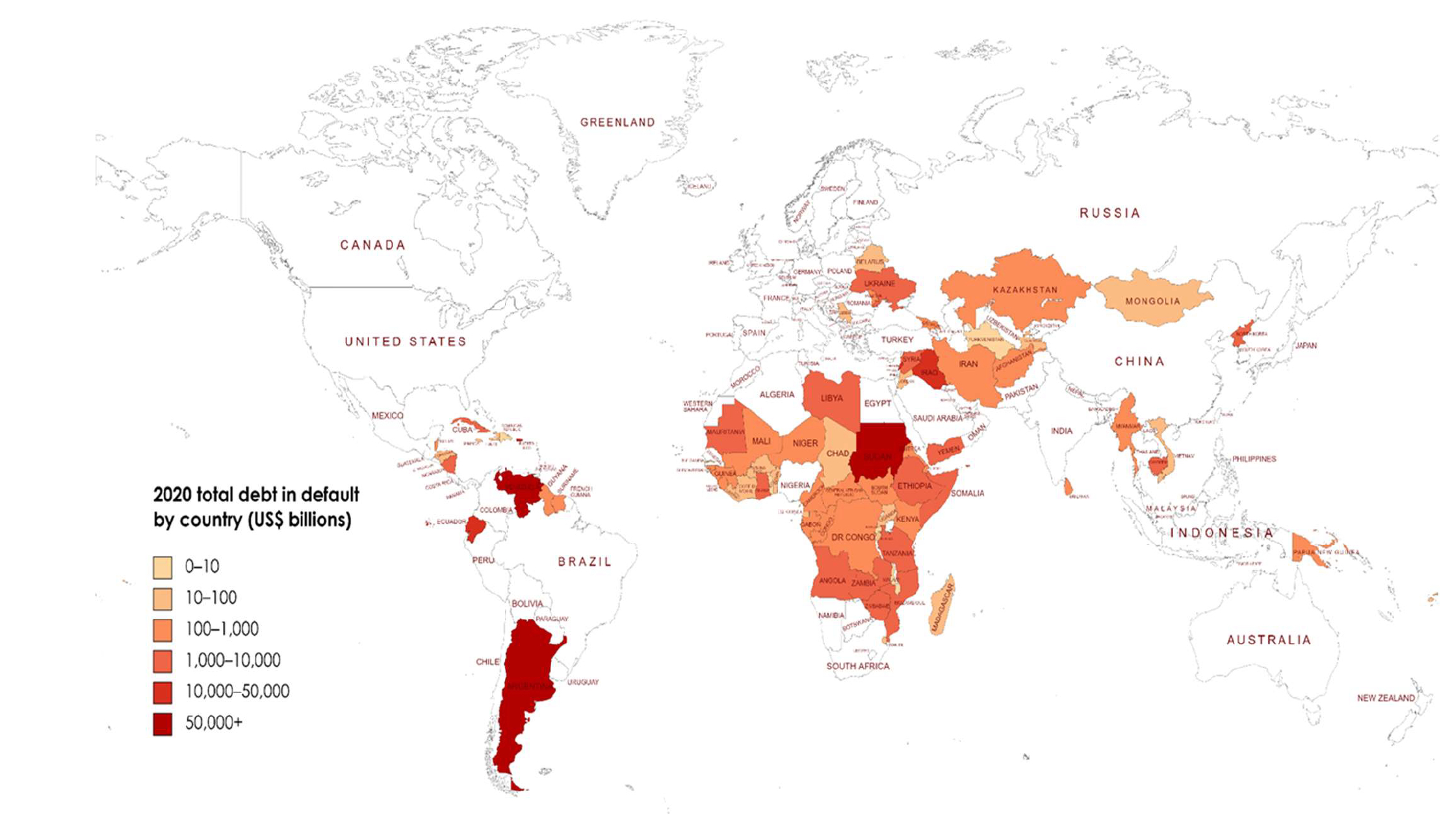
For investors, the most direct measures of country risk come from measures of their capacity to default on their borrowings. At the start of 2022, for instance, there were several countries that were in technical default, on at least portions of their debt, and the Russian invasion of Ukraine has exacerbated sovereign default concerns around the world:
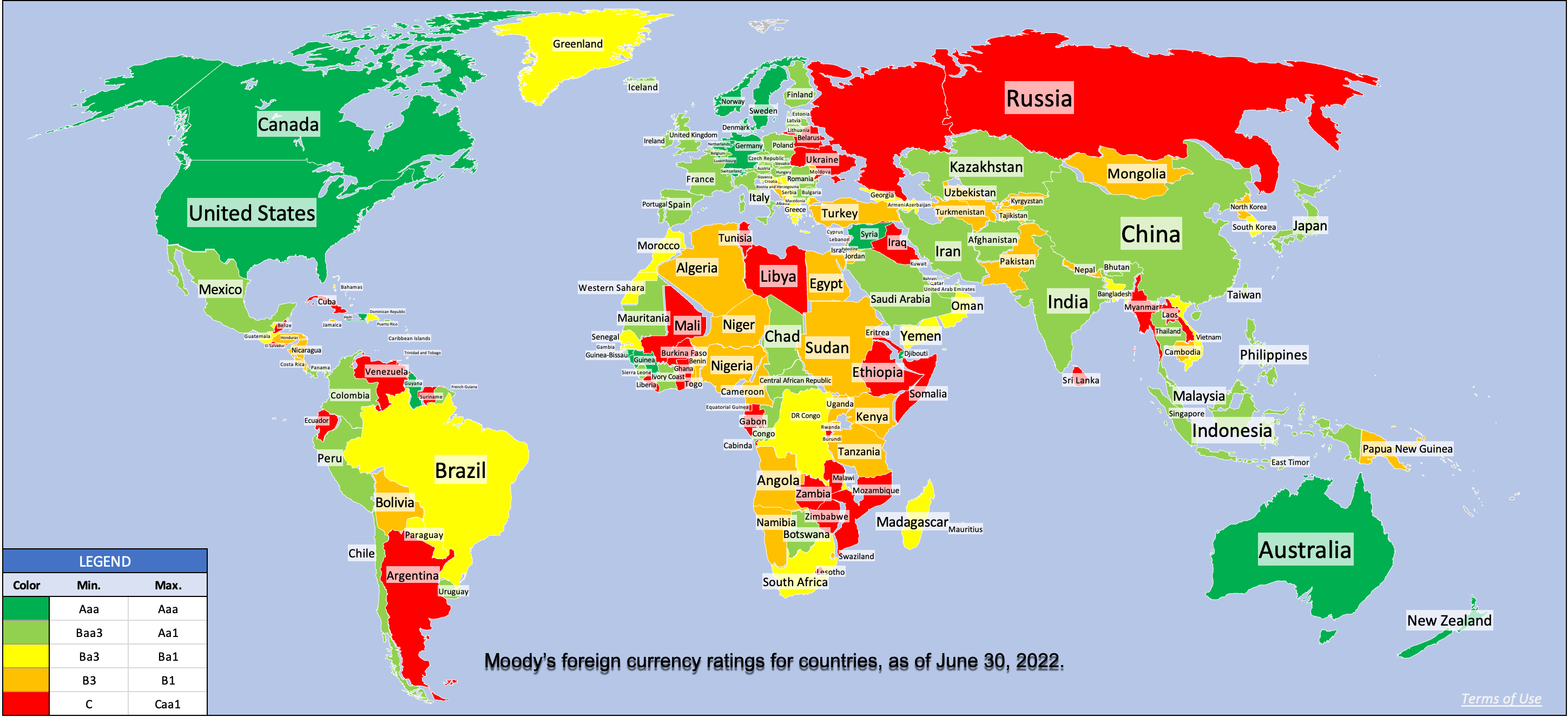
To measure sovereign default risk, ratings agencies (S&P, Moody’s, Fitch) estimate sovereign ratings for countries, designed to capture risk exposure in both local and foreign currency borrowing. The picture below reports on Moody’s ratings, as of June 30, 2022:
Note that this picture has been updated to incorporate Russia’s rating reassessment (downgraded to Ca in early April, before the rating was entirely withdrawn). I know that there are some of you, who distrust ratings agencies, arguing that they have regional and other biases and/or that they do not adjust ratings in a timely fashion. If you are in that group, the sovereign CDS market offers market-based and real-time measures of sovereign default risk, although for only 80 countries, and the map below reports the sovereign CDS spreads, as of June 30, 2022:
Source: Bloomberg
Comparing the sovereign CDS spread picture to the sovereign ratings picture, you can see the overlaps, with the ratings agencies and CDS market mostly in agreement.
Country Risk: Equity Risk
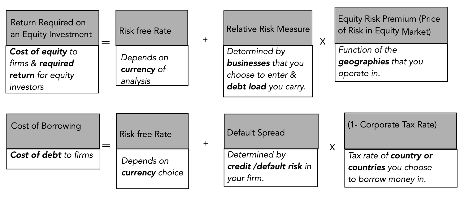
For equity investors, the price of risk is captured by the equity risk premium, and equity risk premiums will vary across countries. I use a template that starts with the implied equity risk premium that I compute for the S&P 500 and then adds on a country risk premium that is computed based upon the sovereign default spread (either from the CDS market or based upon a sovereign rating), to get equity risk premiums for countries:
The equity risk premiums that result from this assessment are shown in the picture below, with a very rough attempt to break down countries geographically. (Please do not attach any political significance to my country groupings, or take them personally. I mean no disrespect to any country, and if you feel your country has been mis-grouped, I apologize.):
If you compare the numbers in this picture to the equivalent one that I reported at the start of the year, you can see the surge in risk premiums across the board, starting with a higher base premium (6.01%, up from 4.24%) for the US and higher spreads for country risk. Looking at individual countries, the graph below summarizes the countries that saw the biggest increases in equity risk premiums (on a percentage basis) over the six months (from Jan 1, 2022 - June 30, 2022):
Not surprisingly, Russia and Ukraine make the list, with Russia's equity risk premium almost tripling and Ukraine's doubling over the period, but you can see the spillover effects into Belarus and Kyrgyzstan. There are three African countries that make the list (Namibia, Mali and Ghana), largely because of ratings downgrades, Sri Lanka's downgrade reflects the implosion of its political system and El Salvador's experiments with Bitcoin are not going well.
Country Risk: Currency and Cost of Capital
As a final part to this post, to see the shifts in country risk that we have seen in 2022, let’s start with an assessment of risk free rates. In my last post, I noted that concerns about inflation have played a big role in pushing up the US ten-year treasury bond rate from 1.51% on Jan 1, 2022, to 3.02% on June 30, 2022. That increase in interest rates is not restricted to the US dollar, as local currency government bond rates have risen around the world. In the graph below, I use these government bond rates as a starting point to estimate riskfree rates in multiple currencies, with adjustments for default risk in governments, using the sovereign default spreads from the last section:
The biggest reason for differences in risk free rates across currencies is differences in expected inflation, with higher inflation currencies exhibiting higher riskfree rates. That said, the key to dealing with currency appropriately in valuation is to stay consistent, with cash flows and the discount rates incorporating the same expectations of inflation:
In short, changing the currency that you use to value a company should not fundamentally change your assessment of that company’s value, and the reason that it often does in practice is because analysts are often sloppy in their treatment of currency, mixing growth rates in one currency with discount rates in another, and real with nominal numbers. As a general principle, to prevent double or miscounting inflation effects and risk, each input into discount rates carries a specific component, with the riskfree rate being the conveyor of expected inflation, the relative risk measure (beta for equity, bond rating for debt) measuring the business and leverage risk of the company and the equity risk premium/default spread reflecting the price of risk in markets.
The combination of rising risk free rates (not just in US dollars, but also in other currencies) and surging risk premiums (default spreads and equity risk premiums) is pushing up corporate costs of capital. In the figure below, I graph the costs of capital for US and global firms, in US$ terms, on July 1, 2022:
In January 2022, I had posted a similar histogram of costs of capital for global and US companies, reflecting risk free rates and risk premiums then, and the change, over the six months, has been extraordinary, with the median cost of capital for a US firm increasing from 5.77% to 8.97%, and for a global firm, from 6.37% to 9.70%. As I look across the many posts I have had this year on how inflation is changing market pricing and psychology, I find myself drawing on one of my favorite Bob Dylan lyrics, "the times, they are a'changin'". The biggest risk that we face, as we navigate our way through uncharted territory, is inertia, where we continue to do the things that have worked for the last decade, when we need to adapt and change.
In any version of a risk and return model for discount rates, where you start with a riskfree rate as a base and build up to costs of equity, debt and capital, it seems blindingly obvious that as interest rates go lower, discount rates will follow and that value will increase. It is this logic that has led to the hand wringing about how central banks have both created pricing bubbles and made discounted cash flow valuations implode by “lowering’ rates. In a recent article, Sanford Bernstein proclaimed DCF all but dead in a world with near-zero risk free rates, because as they see it, the resulting low discount rates were pushing up the value of future cash flows, and since these cash flows are inherently more difficult to estimate, DCFs were less reliable. I have no problem with Bernstein's equity research analysts abandoning DCF and switching to pricing stocks instead, but I believe that they need to do it for the right reasons, not the ones outlined in that thought piece.
Risk free Rates in a Static World
A few months ago, I posted on the hubris of central bankers who (a) believe that they control the level of interest rates and (b) that by changing the level of rates, they can affect stock/bond prices as well as real investments at companies. It is this misguided view of the world that, in my view, has given us years of ever-lower central banking rates, without the promised for results (of more capital investment and higher real growth). It is instructive that almost a decade into quantitative easing, the global economy still seems to be struggling to find its footing.
Unfortunately, this delusion that you can change the risk free rate and leave all else in the process unaffected is not restricted to central bankers and seems to have spread like a virus among valuation analysts, leading to many following the Bernstein script and abandoning DCF. The mathematics are impeccable. If you leave risk premiums (equity risk premiums and default spreads) unchanged, hold on to old growth rates and lower just the risk free rate, you will see value increase as the risk free rate decreases and perhaps approach infinity at really low or negative risk free rates.
To see why, let's assume that you had valued a company in 2007, when the risk free rate was close to 4% and the equity risk premium was also 4% and that you had assumed that this company's cash flow to equity, $100 million in the most recent year, would grow at 10% a year for the following five years and 4% thereafter. The value that you would obtain in a DCF would be $3.378 billion. Now assume that you have been revaluing the company every year in the years since, keeping the rest of your parameters fixed and changing just the risk free rate. As the risk free rate has dropped to levels not seen in recent history, your valuations will have zoomed:
Your value of this company increase from $3.4 billion to $9.1 billion , as the risk free rate dropped to 1.5%, and lowering the risk free rate further will only increase value. In fact, at a 0% risk free rate (which is where the Euro and the Swiss Franc are at in November 2016), your valuation would approach infinity. As an added feature, as your risk free rate decreases, a greater proportion of your value comes from the terminal value, accounting for almost 94% of your value at a 1.5% risk free rate compared to 84% of value at a 4% risk free rate. That is the crux of the Bernstein argument against DCF, with the twist that estimating future cash flows is always difficult and that lower risk free rates have tilted valuation towards cash flows even further into the future.
Risk free Rates in a Dynamic World
Let's get real. When risk free rates change substantially, it is not because central banks will them to be lower or higher, but because of shifts in the fundamentals, and those shifts will affect your other inputs into valuation. In this section, I aim to start by showing how changing risk free rates affect growth rates and risk premiums and then argue that the value effect of a change in the risk free rate can be complicated (as market watchers have found out over the decades).
Risk free Rates and Growth (Real and Nominal)
If you have read my prior posts on interest rates and central banks, one of my favorite tools for understanding interest rates is the Fisher equation, which breaks down a riskless rate into two components: an expected inflation rate and an expected real interest rate. Using a proxy of real GDP growth for the real interest rate, I derive an "intrinsic" risk free rate as the sum of the inflation rate and real GDP growth. I may be stretching but it works surprisingly well at explaining why interest rates move over time, as evidenced in the graph below, where I compare the T.Bond rate to the sum of inflation and GDP growth each year from 1954 to 2015.
So, what's the point of this graph? In addition to emphasizing the fact that central banks can affect rates only at the margin, it brings home the reality that low interest rates are indicative of a market that expects both inflation and real growth to remain low. It is entirely possible that the market is wrong but if you are doing valuation, you cannot selectively override the market on one variable (growth in the static example) while holding on to it on the other (risk free rate).
Dynamic Implication: As the risk free rate changes, your estimates of nominal growth will have to be stepped down, not because you have changed your beliefs about a specific company, but because you should be lowering the base growth rate for the economy (global or domestic).
Risk free Rates and ERP
The second variable that goes into play when risk free rates change is the equity risk premium. Again, you have to let go of the notion that equity risk premiums are static numbers that come out of historical data but are reflections of market worries about the future and investor risk aversion. Not surprisingly, the same forces that cause interest rates to move also affect the market's perception of risk and will cause equity risk premiums to shift. This can be seen when you look at implied equity risk premiums, where you back out what the market is demanding as an expected return on stocks from cash flows and subtract the risk free rate. In the graph below, I outline this effect since 2008.
The most striking finding, at least for me, is how little the expected return on stocks has changed since 2008, staying around 8%, while risk free rates have more than halved. The net effect is that the equity risk premium, close to 4% prior to 2008, has now moved to 6% and above.
Dynamic Implication: As the risk free rate changes, the equity risk premiums you use will also have to change to reflect the market's updated expectations. A crisis that causes rates to plummet will also make risk premiums rise. If you stick with historical risk premiums, while using current risk free rates, you will misvalue companies.
Risk free Rates and Default Spreads
The same forces that cause equity risk premiums to rise as risk free rates drop also come into play in the bond market in the form of default spreads on bonds. In the graph below, I estimate the default spread on a Baa rated bond by comparing the Baa bond rate to the T.Bond rate each year from 1960 to 2015.
As with the equity risk premium, default spreads have widened since 2008, from 2.02% in 2007 to 3.23% in 2015.
Dynamic Implication: As the risk free rate changes, the default spread used to estimate the cost of debt should also change, thus ensuring that the cost of debt will not move in lock step with the risk free rate.
Risk free Rates and Debt Ratios
To complete the story, the final ingredient that you need for the cost of capital estimation is a debt to capital ratio in market value terms. If as risk free rates change, both the equity risk premium and default spread also change, it should come as no surprise that the relative benefits of using one (debt) over the other (equity) will also shift. To chronicle these change, I looked at the aggregate debt to capital ratios, in market and book value terms, for all US stocks, each year from 2000 to 2015.
If you divide the time period into pre-2008 higher risk free rate and post-2008 lower risk free rate sub periods, it seems quite clear that US companies are borrowing more money than they used to. The facile explanation is that this is exactly what you would expect with lower interest rates but remember that those lower rates feed into both the cost of equity and debt. This effect is a more subtle one and reflects the relative risk premiums for equity and debt, perhaps suggesting that the price of equity risk has risen more than debt risk.
Dynamic Implication: As the risk free rate changes, the debt ratios for companies will also change as they reevaluate the trade off of using debt as opposed to equity. That change, in conjunction with tax and default risk assessments, will lead to a change in the cost of capital.
Risk free Rates and Value: The Full Picture
Now that we have a fuller picture of how risk free rates are interconnected to risk premiums and growth rates, let me revisit the example that I initiated in the static world of valuing equity in a company with a base year cash flow to equity of $100 million. Rather than let the growth rates and the risk premiums stay unchanged, here is what I assumed:
The nominal growth rate in the economy will be equal to the risk free rate, reflecting how closely the T.Bond rate has tracked the nominal GDP growth rate.
The company will grow at a rate 6% higher than the nominal growth rate of the economy for the next five years. Thus, with a 4% riskfree rate, the growth rate is 10%, matching the original assumption, but at a 2% riskfree rate, the nominal growth in cash flows will be 8%. In perpetuity, the company will now grow at the riskfree rate = nominal growth rate of the economy,
The equity risk premium is the trickiest component, but if the market's behavior over the last decade is any indication, the expected return on stocks will stay at 8%, with the equity risk premium adjusting to the new risk free rate. Thus, if the riskfree rate drops to 2%, the equity risk premium will be 6%.
The effect on value of changing the growth rate is captured in the picture below:
Note that the neither the value nor the percentage of the value from terminal value change much as the risk free rate drops; in fact, they both decline marginally. Furthermore, I can now explore the effect on value of having a zero or negative riskfree rate and it is benign.
I can only give you my personal perspective on how lower interest rates have affected my valuations. With lower rates, contrary to the Bernstein thesis, I find myself less worried about terminal values and the assumptions that I might have made incorrectly. When my nominal growth rate in perpetuity is capped at 2%, 1% or even 0%, I can do far less damage with my assumptions about what a firm can do in perpetuity, than I did in 2007. If anything, low risk free rates makes my intrinsic valuations less volatile, not more so. It is true that these are dangerous times for auto-pilot DCFs where a combination of inertia, trust in historical data (on risk premiums and growth rates) and failure to check for internal consistency can lead to explosively bad DCFs. If Bernstein's point is that a good pricing (based upon multiples and comparable firms) is better than an auto-pilot DCF, I am in agreement!
Playing Devil's Advocate
If you are skeptical about my arguments, I don't blame you! In fact, I will preempt you and bring up some counter arguments that you can make against my thesis.
Mean Reversion: The essence of mean reversion is that when something looks unusually low or high, it will be revert back to historic norms. Using this argument on risk free rates, there are some who use "normalized" risk free rates (with the extent of normalization varying across users) in valuation. There are two problems with this argument. The first, and I referenced it in a different context in my post on CAPE, is that assuming things will revert back to the way they used to be can be dangerous, if there has been a structural shift in the process. The second, and perhaps even stronger, argument is that you cannot selectively mean revert some numbers and not mean revert others. Thus, if you decide to replace today's risk free rate with a normalized risk free rate of 4%, reflecting 2007 levels, you have to also adjust your growth rates and risk premiums to reflect 2007 levels. In effect, you will be valuing your company in 2016, as if your were back in 2007. Good luck with that!
Central Bank as Master Manipulators: The conventional wisdom is that the Fed (and central banks) are all-powerful and that the low rates of today have little to do with fundamentals and more to do with central banking policy. If you believe that and you also believe that markets are being led by the nose, you do have the basis for a "bubble" argument, where "artificially" low interest rates are leading all financial assets into bubble territory. The problem, though, is that if this were the case, the cost of equity should be tracking down, in step with the risk free rate, and as the figure on equity risk premiums (in the section above) notes, that does not seem to be the case.
That is not to say that I am sanguine about low interest rates. The low growth and low inflation that these numbers signal are having their effect on companies. Real investment has declined, cash flows to investors (in dividends and buybacks) have increased and cash balances have surged. The increase in debt at companies will not only increase default risk but make these companies more sensitive to macro economic shifts, with more distress and default coming in the next downturn. Finally, to the extent that central banks send signals about the future, the desperation that is being signaled by their policies does not evoke much confidence in them.
Conclusion
The risk free rate is an input into a discounted cash flow valuation but it is not an input that can be changed in isolation. When risk free rates change, they reflect shifts in fundamentals that should also show up in risk premiums and growth rates, making any resulting change in value difficult to forecast. As the hysteria mounts ahead of the next FOMC meeting, my suggestion is that you step back and take a big-picture perspective. This too shall pass!
In discounted cash flow valuation, discount rates are the instruments that we use to adjust for the risk in cash flows. In practice, discount rates often take on a far greater role. Some analysts use them to bring in the quality of management, pushing down discount rates for what they perceive as well-managed firms and pushing up discount rates for poor management. Venture capitalists pump up discount rates to compensate themselves for failure risk, i.e., that many of the firms that they invest in will not make it. While these adjustments may seem intuitive, they are dangerous for many reasons: you can double count both the good and bad, you may be adjusting for risks you should not be and biasing your valuations.
Management Quality, Competitive Advantages and Discount Rates
It remains almost an act of faith in some old-time value investing circles that the rate of return that you should demand on an investment (or discount rate) should reflect the quality of its management and competitive advantages (or moats). Though this seems intuitive, it is not true for a simple reason. Management quality and moats will affect the expected earnings and cash flows, with better quality management and bigger moats delivering higher earnings and cash flows (than for firms without these qualities) but the relationship with risk and discount rates remain tenuous, at best. That is because risk has to do with uncertainty about levels, rather than levels.
To see why, consider two companies with vastly different management in the same business. Company A, with “high quality” managers in place is aggressive in its pursuit of growth while also being discriminating, a rare combination that delivers an expected operating margin of 8%, with high variability, with values ranging from 5% to 11%. Company B has a management team whose governing style is inertia, delivering sub-par margins of 3% but with much less variability (2.5% - 3.5%). In this example, company A will have a higher cost of capital than company B but with its higher cash flows, it will also be worth a great deal more. In fact, intuition leads me to believe that companies with significant competitive advantages (moats) and high barriers to entry are often more risky, since the loss of these competitive advantages will cause a much greater loss in value than for companies that are expected to tread water and earn close to their cost of capital.
Risk and Discount Rates
When valuing companies, you confront all kinds of risk, some related to the company and some to the macro economy, some continuous and some discrete. In my post on uncertainty, I broke risks down in different categories and the way you incorporate risk into value can depend on the type of risk. While it does seem intuitive to use the
discount rate as the receptacle for all the risks that you are exposed to, it
does not work very well. The reason is simple. A DCF is a going concern concept and the
discount rate is designed to capture risks to a going concern, i.e., risks that
cause revenues, earnings and cash flows to change over time but not truncation
risk, i.e., risks that can cause an end to a company’s life. If you add on the perspective of a diversified investor looking at the going concern, the risk that is incorporated into a discount rate should only be macroeconomic risk that affects the value of the firm as a going concern and neither truncation risk nor micro/estimation risk has a place in value.
So what should be done about risks like nationalization risk or distress risk? While your discount rate may be ill-equipped to convey theses risk, they should have an effect on value and I borrow a tool from probability & statistics to capture this effect.
Decision
Trees and Truncation Risk
By attaching a probability to the truncation
risk and calculating the consequence, you will reduce your expected value for
an asset without doing discount rate gymnastics. That is the technique that I
would use to value a start-up (with a high risk of failure), a young biotech
company (where the failure to get drug approval can cause it to shut down) or
even a large bank with a regulatory capital problem and the possibility of an
equity wipeout (see my Deutsche Bank valuation from a couple of weeks ago). If you are interested in extending your probabilistic arsenal, try this paper that I have on the topic.
What about company specific and estimation risk? Uncomfortable though it may make you to do so, when valuing public companies that are at the margin priced by institutional and diversified investors, you should let these risks pass through and use diversification as your tool for averaging risk. As for the oft-touted advice that the cash flows should be adjusted for risk, I would advice caution since many people who offer this advice seem to think that estimating cash flows across many scenarios and taking an expected value across them is adjusting for risk. It is not!
The Distractions
In any discussion of discount rates, distractions abound that can lead you not only away from good sense but very quickly into a morass. Here are three of the most common distractions:
Margin of Safety: Many investors tout the margin of safety as their protection against risk. While I have absolutely no issue with building in a margin of safety into your investment decisions, as long as you recognize that there is a cost to being too conservative, I do not believe that it can be offered as an alternative to risk-adjusting the discount rate. As I understand it, the margin of safety is the buffer you build between value and price to protect yourself against your mistakes. If you are using a DCF to estimate value, you still need a risk-adjusted discount ate.
Homework: When doing valuation, I have been sometimes told that the reason that I face risk is because I have not done my homework, and that spending more time understanding the company, its business and the management will make the risk go away. Really? So, when valuing a Brazilian company, all I have to do is spend more time with the numbers and Brazil's political and economic uncertainties will magically vanish? I don't think so!
"But Warren Buffett says": I have been told that Warren Buffett not only abhors the use of betas in valuation (and I dealt with that concern in Myth 4.2) but uses the risk free rate as his discount rate in valuing companies. Before you jump to the conclusion that he does not adjust for risk, I believe that his way of adjusting for risk is to count only that portion of a company's earnings that is predictable. In effect, he is using what I would call "certainty equivalent" cash flows. That approach may work reasonably well with mature companies but will quickly break down for growth companies.
You can always choose another tool for estimating intrinsic value, but if you use a discounted cash flow valuation to estimate value, you have to estimate expected cash flows, adjust the discount rate for going concern risk and arrive at a value.
Conclusion
When doing discounted cash flow valuation, the discount rate exerts a pull on analysts, inviting them to use it as a receptacle for their hopes and fears. Doing so will expose you to double counting both the good stuff (great management, strong moats) and the bad ones (exposure to catastrophic risk, concerns about uncertainty). The discount rate, at least in a DCF, is meant to carry the weight of measuring going-concern risks and that too from the perspective of the marginal investors in the company. That is task enough and it is best not to load it up with much more! YouTube Video
In my last post, I argued that academics and practitioners pay too much attention to discount rates in valuation and too little to cash flows. One reason for that attention may by the fear that you have only one shot at estimating the cost of equity or capital, when valuing a firm, and that once estimated, that number becomes the discount rate to use on cash flows in perpetuity. In this post, I will argue that this fear is misplaced and that the DCF approach not only allows for changing discount rates over time but requires it for most firms.
The Mechanics of Time-varying Discount Rates
In a discounted cash flow valuation, the value of an asset is the present value of the expected cash flows, with the equation written as follows:
Written in this form, the “r” in the denominator is the discount rate and is estimated as the cost of equity (or capital), depending on the cash flows that are being discounted. In practice, analysts seem to operate under the presumption that they get one shot at estimating these discount rates, at the start of the process, and that these discount rates are then fixed in perpetuity. That presumption is wrong, since the DCF structure is flexible enough to allow for time varying discount rates, with the modified version of the value equation below:
Note that r1 is the discount rate for year 1, r2 is the discount rate in year 2 and so on until your get to your terminal value and the discount rate in perpetuity is rN. There is one minor computational detail which can have major valuation effects. Note that, in the presence of time varying discount rates, the way we do discounting changes. Rather than discount back each year’s cash flow at that year’s discount rate, we compute a compounded discount rate in each period. Thus, if your cost of capital is 12% in year 1, 11% in year 2 and 10% in year 3, the present value of $100 million in year 3 is as follows:
If this cash flow had been discounted back (by mistake) at 10% for 3 years, the present value would have been (wrongly) computed to be $75.13 million. Intuitively, you are adjusting the present value of cash flows later for the risk that you have to live through in the earlier years.
The Intuition for Time-varying Discount Rate
Adjusting discount rates across time may seem like a needless complication but it is a necessary one, if you want your valuation to remain internally consistent. More specifically, if you are assuming changes in your company characteristics (growth, business mix, geographical exposure) in your cash flows, as you move through time, you should be changing the discount rate to reflect these changes.
While this is true for all companies, the effect will be greater when you are valuing young companies or companies in transition, where you expect large changes in the company as you move through your forecast period. Thus, in my valuations of Uber in 2014 (a young growth company) and Tesla in July 2016 (a growth company in transition) & Apple in 2016 (a mature company with solid cash flows), my discount rates changed over time.
How much do these changing discount rates affect the values per share? Considerably, as can be seen in the graph below where I contrast the values that I would have obtained for the three companies with my default assumption of changing discount rates with the values that I would have obtained if the discount rates had been left at the starting levels.
Value with time-varying Discount Rate
Value with constant discount Rate
Effect on value
Uber (June 2014)
$5,895
$3,601
-38.91%
Tesla (July 2016)
$22,364
$17,688
-20.91%
Apple (May 2016)
$692,852
$633,336
-8.59%
With Uber, the effect on value is substantial, increasing the value of equity by almost 39%, with Tesla the effect is smaller (21%) and with Apple, even more muted (8.6%).
Guidelines for Discount Rate Adjustments
If you buy into the argument that the costs of equity and capital can change over time, it may seem like that your estimation problems have multiplied, since you now have to not only estimate the current cost of capital for a firm but costs of capital every year through your valuation. To simplify the estimation process, here is what I find works for me:
To estimate the cost of capital that you will use in the early years (years 1 and 2), start with the current cost of capital for the firm. That will reflect the existing business mix for the firm (in the beta), the geography of its revenues (in the equity risk premium) and the debt policy for the firm (in the cost of debt and debt ratio).
If the company has clearly specified plans to change its debt ratio and business mix in the near term, adjust the cost of capital for these changes in the near years (years 3-5) for these changes. If it does not, leave the cost of capital at the current level.
The cost of capital in steady state (for terminal value) should move towards those of mature firms. If you see your firm growing across multiple businesses, that cost of capital should be that of the market (with a beta of one, a debt ratio close to the market average) but if you see it growing within only its existing business, the cost of capital should be reflecting of the industry average (reflecting the industry average beta and debt ratio).
In the transition period (between the near years and steady state), you should adjust the cost of capital from your near-year level to stable growth levels, using linear increments.
Phase
Forecast years
Beta
Equity Risk Premium
Debt Ratio
Cost of debt
Start of valuation
Yr 1-2
Reflects current business mix
Current geography of operations
Current market debt ratio
Current bond rating or default risk assessment
Build up
Yrs 3-5
Changes in business mix (if any)
Changes in geography (if any)
Targeted debt ratio (if any)
Default risk, given new debt ratio
Transition
Yrs 6-10
Move incrementally to stable period beta
Adjust to stable period ERP
Adjust to stable period debt ratio
Adjust to stable period cost of debt
Stable growth (Steady State)
Year 10 & beyond
Move to 1, if company grows across businesses, or to industry average, if it stays within business
Steady state geographic exposure and equity risk premium estimates for long term.
Market-average debt ratio (if growth across businesses) or industry-average debt ratio (if single business)
Stable company cost of debt
One reason that I compute the costs of capital, by industry grouping, and update it each year is to have access to this information whenever I value a company. If you are interested, you can find the industry average costs of equity and capital for US firms and global firms on my website.
If you open the door to adjusting discount rates for changes in company characteristics, you can also consider also bringing in changes in the macroeconomic inputs. In particular, you could allow the risk free rate and risk premiums (in the form of default spreads and equity risk premiums) to change over time, and as they do, so will your discount rate. Thus, if you believe, as many do, that risk free rates are “too low” (given fundamentals) but are wary of replacing actual rates with your estimates, you could have your cake and eat it too, by starting off with current risk free rates and adjusting those rates to what you believe are more normal levels over time. If you do so, though, you should also normalize equity risk premiums and default spreads over time. To provide an illustration, consider the cost of equity for an average-risk (beta =1_ company in US dollars in October 2016, with the US dollar risk free rate at 1.6% and the mature market equity risk premium at about 6%.
Let’s assume that you believe that the risk free rate should be closer to 3%, given inflation and real growth today, and that you believe that the market rate will move towards this number over the next decade. Let’s also assume that you also believe that as risk free rates normalize, the equity risk premium will move back towards its average over the last decade (about 5%) The cost of equity for your company ten years from now (which you will use in your terminal value calculation) will then be 8%:
Cost of equity in year 10 = Expected Risk free rate + Beta (ERP) = 3% + 1 (5%) = 8%
If you are a company with substantial emerging market exposure (say in India or Brazil), you may also be adjusting the additional country risk premium that you incorporate into your cost of equity over time.
Conclusion
One reason that analysts often feel helpless, when computing intrinsic value in a DCF, is because they feel that they not only have little control over the discount rate, since all the inputs come from outside, but that they are stuck with this discount rate forever. If your discount rates adjust over time to reflect changes in your company, towards industry or market averages, these rates will start to have a smaller effect on your valuations and that is not only healthy but more realistic (at least in my view).
If you have taken a class on valuation, think back to what you spent most of your time doing and I will wager you spent it talking about discount rates. If there was any attention paid to cash flows and growth, it was either cursory or mechanical, and perhaps as a set up to returning to the discount rate discussion. I blame both practitioners and academia for this focus. The practitioner obsession with discount rates can be seen both in the time spent talking about discount rates at conferences and on estimating it in valuation. Reviewing the academic literature over the last few decades, the preponderance of it has been focused on developing models to estimate expected returns on risky investments (discount rates). As a result, classical portfolio theory and discounted cash flow valuation have become so entangled that, as I noted in my last post, there are those who on losing faith with portfolio theory have also felt the need to abandon DCF valuation as well.
The Discount Rate Obsession
Why are we so focused on discount rates in valuation? One reason is that we attribute more consequence to getting it wrong than we should, partly because of the very first valuation models that we are exposed to. The other is that spending time on the inputs into discount rates gives us a false sense of both control and precision.
The roots of discounted cash flow valuation, at least as practiced today, can be traced back almost 80 years to a treatise by John Williams on value, but its popular usage was tied to the development the Gordon Growth Model, where it was simplified for use with dividends in constant growth.
Note that this simplified equation is built on two assumptions: that companies pay out what they can afford to (excess cash) in dividends and that these dividends can grow at a constant rate forever. In this model, it is easy to see why the valuation exercise becomes one of estimating discount rates since the dividends are known and the growth rate is constrained to be less than equal to the economy. In fact, staying with the constant growth model, which is how the terminal value is estimated in more expansive versions of the DCF (with free cash flows replacing dividends and high growth periods as front ends to the terminal value), the effect of changing the discount rate on value can be considerable. To illustrate this, I estimate the value per share for a company that is expected to pay a dividend per share of $1.00 next year, growing 3% a year in perpetuity, for costs of equity (discount rates) ranging from 4% to 10%.
No wonder estimating discount rates paralyzes analysts, since getting it wrong could lead you to value a $16.67 stock (if 10% is the right discount rate) at $100 (if you use 4% as the discount rate).
There is also a behavioral component at play in the discount rate focus. When faced with significant uncertainty in valuation, it is comforting to turn our attention back to discount rates, where we can draw on established models and data to estimate and fine tune the components (risk premiums, betas, costs of debt). Estimating risk free rates, betas and equity risk premiums to the second, third or even fourth decimal points offers the illusion of control in a world where estimates of revenue growth and operating margins are difficult.
The Cross Sectional Distribution of Cost of Capital
Is the focus on discount rates merited? How important is it to get the discount rate right? To answer that question, it is best to look at the numbers. At the start of 2016, as I have at the start of each of the prior years, I estimated the costs of capital for individual companies in a process that I described more fully in this post. The graph below provides the distribution of costs of capital, in US dollars, for US companies at the start of 2016:
The most striking feature of this graph is the bunching together of costs of capital around 8.5%, with half of all companies having costs of capital between 6.6% and 9.20%. Expanding the sample to look at all 41,889 companies listed globally, you do get a wider distribution, even in US dollar terms, as you get bigger differences in country risk play out in the computation.
Even in this broader sample, the costs of capital, in US $, of most global companies lies in a tight range, with 50% of companies falling between 7.43% and 10.15%. Moving to other currencies will cause the costs of capital to change, not because there is currency risk, but because of differences in inflation. Thus, the range for cost of capital, in Indian rupee terms, allowing for an inflation differential of 5% with the US dollar, would mean that the range in rupee terms will be 12.43% to 15.15% for half of all global companies.
Conclusion
Instead of spending most of our time during valuation estimating discount rates and debating how best to measure risk, as we are prone to do, we will be better served spending more time estimating expected cash flows and growth rates, since big mistakes in valuation are more likely to be made there. While I would make this statement about any company, it is particularly true for younger companies and in the face of uncertainty about the future. In fact, let me propose a compromise. If you have to value a US company in a hurry, why not just use a cost of capital of 8% in July 2016, the median value for US stocks, and spend your limited time on the numerator (cash flows)? YouTube Video
Let’s start by stating the obvious. You need a D(iscount rate) to do D(iscounted) C(ash) F(low) valuation. To get that discount rate, I use a beta to estimate a cost of equity (and cost of capital) in my valuation and it is that input that evokes the biggest backlash from people perusing the valuation. Many investors have a visceral mistrust of anything that emerges from portfolio theory and betas to them symbolize what they see as the academic view of valuation. Consequently, not only do they take issue with the discount rates that I use in my valuations, they often choose not to do discounted cash flow valuation, because of their discount rate disagreements. Talk about throwing the baby out with the bathwater!
The D in the DCF: Big Picture Perspective
To understand the role that the discount rate plays in discounted cash flow valuation, it is worth going back to the DCF equation for the value of an asset with a life of n years, with expected cashflows (E(CF)) in each time period in the numerator and the discount rate (r) in the denominator.
Note that in a conventional DCF, the numerator has expected cash flows (across all scenarios, good and bad) and it is the denominator (the discount rate) that carries the burden of adjusting for risk. In the context of valuing a business, this risk-adjusted number can take two forms, depending on how the valuation is structured.
You can stay equity-focused, estimate cash flows to equity (dividends or potential dividends) and discount back at a risk-adjusted rate of return demanded by equity investors (the cost of equity) or you can value the entire business, discounting cash flows to both equity investors and lenders (a pre-debt cash flow) at a weighted average of the cost of equity and the cost of debt, with the latter adjusted for tax benefits on borrowing. If you take the latter path, the discount rate, in addition to carrying the weight of reflecting the risk in your operations now also carries an added burden of incorporating the value added or destroyed by your financing choices (captured in your costs of debt, equity and capital). Note that a DCF model is agnostic about the process that you use to estimate the discount rate and does not require any specific model (with our without betas). Estimating
Discount Rates – The Portfolio Theory Construct
The question that you face in valuation then becomes how best to estimate the discount rates (costs of equity & capital), given the fact that they are not easily observable. The advent of portfolio theory in the 1950s and the subsequent development of the capital asset pricing model in the next decade have been both a boon and a bane for discounted cash flow valuation.
The groundbreaking insight that Harry Markowitz brought to this process was his recognition that the risk in an investment can look very different to one who has all of his or her money in that investment than from one who has his or her money spread across multiple investments. Looking at risk through the eyes of a diversified marginal investor not only changes our definition of risk (to risk that cannot be diversified away) but allows us to measure it with a beta (in the CAPM) and with betas (in multi-factor and arbitrage pricing models), offering pathways to estimating costs of equity for companies.
Risk and Return Models: Modern Portfolio Theory
Model
Assumptions
Risk Measure
The CAPM
(1) There are no transactions costs.
(2) There is no private information.
The marginal investors will be fully diversified and hold a portfolio of every traded asset in the market. The risk of an individual asset will be captured by the risk added to this market portfolio, and estimated with a single beta, measured against the market.
The APM
The market prices of stocks are the best indicators of market and firm-specific risks, with market risks affecting all or many stocks and firm-specific risks not.
Historical stock returns can be analyzed to identify the market risk factors and the exposure of each stock to those factors. Since this is a statistical model, the factors will be unnamed. The risk in a stock will be captured with betas, measured against these unnamed factors.
The Multifactor Model
Market risk factors have to be macroeconomic, to affect many stocks at the same time. Looking at how a stock behaves, relative to different macroeconomic variables, should yield clues to its market risk exposure.
The risk in a stock will be captured with betas, measured against specified macroeconomic factors.
Easier access to stock price data has allowed us to estimate the beta or betas for individual companies, leading us inexorably to where we are today, where cost of capital calculations have become mechanical processes, with inputs being outsourced to services. If you
don’t like betas…
There are many analysts who disagree with the marginal investor assumption and the resulting focus on just non-diversifiable risk. There are perhaps just as many old-time value investors who believe that it is inconsistent to use a price-based risk measure in intrinsic valuation. I see merit in their points of view, but I don't believe that their prescription of abandoning discounted cash flow valuation all together is appropriate. If you are a non-believer in either portfolio theory or in price-based risk measures, there are alternative ways of estimating discount rates that may be more in line with your views on markets, as long as you identify the basis for your disagreement, i.e., whether it is with the assumption that the marginal investor is diversified or with the use of price-based risk measures. The figure below lists the alternatives:
Alternative Models for Risk Measurement
Thus, if your quibble is with the diversified marginal investor assumption, you can use a relative risk measure based upon the total risk in an investment (and not just the non-diversifiable risk), a proxy model for discount rates (where you relate them market capitalization, price to book or price momentum) or even a market-determined implied return (backed out of current prices). If you have issues with price-based risk measures, you should consider using variability in accounting earnings, measures of default risk or even qualitative measures (risk classes or sector-based risk measures) to come up with discount rates.
The
bottom line
In my view, portfolio theory has advanced the
cause of estimating discount rates by introducing three common sense components
into valuation. The first is that the risk in an investment is the risk that it
adds to a portfolio and not based upon it standing alone. The second is that as
small investors, we are price takers, with prices set by the larger investors
(usually institutional and mostly diversified). The third is that there is information in the stock price movements, with volatility in stock prices reflecting
higher underlying risk, than in alternative measures of business performance
(like earnings or cash flows). I will continue to use betas in estimating costs
of equity, while recognizing their limitations and being willing to adapt to
specific circumstances (like valuing private businesses or closely held
companies, where the underlying assumptions are most likely to be violated). If
you disagree with my point of view, you are on solid ground, as long as you
recognize that you will now have to come up with an alternate risk measure that
you can live with. If that risk measure is based upon accounting numbers
(earnings, debt ratio) or on company characteristics (size, sector), you should
recognize that it comes with its own set of problems and be willing to correct
for them. Paraphrasing Milton Friedman, it takes a model to beat a model!