There is a reason that every religion inveighs against borrowing money, driven by a history of people and businesses, borrowing too much and then paying the price, but a special vitriol is reserved for the lenders, not the borrowers, for encouraging this behavior. At the same time, in much of the word, governments have encouraged the use of debt, by providing tax benefits to businesses (and individuals) who borrow money. In this post, I look at the use of debt by businesses, around the globe, chronicling both the magnitude of borrowing, and the details of debt (in terms of maturity, fixed vs floating, straight vs convertible). The tension between borrowing too little, and leaving tax benefits on the table, and borrowing too much, and exposing yourself to default risk, is felt at every business, but the choice of how much to borrow is often driven by a range of other considerations, some of which are illusory, and some reflecting the frictions of the market in which a business operates.
The Debt Trade off
As a prelude to examining the debt and equity tradeoff, it is best to first nail down what distinguishes the two sources of capital. There are many who trust accountants to do this for them, using whatever is listed as debt on the balance sheet as debt, but that can be a mistake, since accounting has been guilty of mis-categorizing and missing key parts of debt. To me, the key distinction between debt and equity lies in the nature of the claims that its holders have on cash flows from the business. Debt entitles its holders to contractual claims on cash flows, with interest and principal payments being the most common forms, whereas equity gives its holders a claim on whatever is left over (residual claims). The latter (equity investors) take the lead in how the business is run, by getting a say in choosing who manages the business and how it is run, while lenders act, for the most part, as a restraining influence.

Using this distinction, all interest-bearing debt, short term and long term, clears meets the criteria for debt, but for almost a century, leases, which also clearly meet the criteria (contractually set, limited role in management) of debt, were left off the books by accountants. It was only in 2019 that the accounting rule-writers (IFRS and GAAP) finally did the right thing, albeit with a myriad of rules and exceptions.
Every business, small or large, private or public and anywhere in the world, faces a question of whether to borrow money, and if so, how much, and in many businesses, that choice is driven by illusory benefits and costs. Under the illusory benefits of debt, I would include the following:
- Borrowing increases the return on equity, and is thus good: Having spent much of the last few decades in New York, I have had my share of interactions with real estate developers and private equity investors, who are active and heavy users of debt in funding their deals. One reason that I have heard from some of them is that using debt allows them to earn higher returns on equity, and that it is therefore a better funding source than equity. The first part of the statement, i.e., that borrowing money increases the expected return on equity in an investment, is true, for the most part, since you have to contribute less equity to get the deal done, and the net income you generate, even after interest payments, will be a higher percentage of the equity invested. It is the second part of the statement that I would take issue with, since the higher return on equity, that comes with more debt, will be accompanied by a higher cost of equity, because of the use of that debt. In short, I would be very skeptical of any analysis that claims to turn a neutral or bad project, funded entirely with equity, into a good one, with the use of debt, especially when tax benefits are kept out of the analysis.
- The cost of debt is lower than the cost of equity: If you review my sixth data update on hurdle rates, and go through my cost of capital calculation, there is one inescapable conclusion. At every level of debt, the cost of equity is generally much higher than the cost of debt for a simple reason. As the last claimants in line, equity investors have to demand a higher expected return than lenders to break even. That leads some to conclude, wrongly, that debt is cheaper than equity and more debt will lower the cost of capital. (I will explain why later in the post.)
- Debt will reduce profits (net income): On an absolute basis, a business will become less profitable, if profits are defined as net income, if it borrows more money. That additional debt will give rise to interest expenses and lower net income. The problem with using this rationale for not borrowing money is that it misses the other side of debt usage, where using more debt reduces the equity that you will have to invest.
- Debt will lower bond ratings: For companies that have bond ratings, many decisions that relate to use of debt will take into account what that added debt will do to the company’s rating. When companies borrow more money, it may seem obvious that default risk has increased and that ratings should drop, because that debt comes with contractual commitments. However, remember that the added debt is going into investments (projects, joint ventures, acquisitions), and these investments will generate earnings and cash flows. When the debt is within reasonable bounds (scaling up with the company), a company can borrow money, and not lower its ratings. Even if bond ratings drop, a business may be worth more, at that lower rating, if the tax benefits from the debt offset the higher default risk.
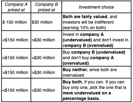
- Equity is cheaper than debt: There are businesspeople (including some CFOs) who argue that debt is cheaper than equity, basing that conclusion on a comparison of the explicit costs associated with each – interest payments on debt and dividends on equity. By that measure, equity is free at companies that pay no dividends, an absurd conclusion, since investors in equity anticipate and build in an expectation of price appreciation. Equity has a cost, with the expected price appreciation being implicit, but it is more expensive than debt.
The picture below captures these illusory benefits and costs:

If the above listed are illusory reasons for borrowing or not borrowing, what are the real reasons for companies borrowing money or not borrowing? The two primary benefits of borrowing are listed below:
- Tax Benefits of Debt: The interest expenses that you have on debt are tax deductible in much of the world, and that allows companies that borrow money to effectively lower their cost of borrowing:
After-tax cost of debt = Interest rate on debt (1 – tax rate)
In dollar terms, the effect is similar; a firm with a 25% tax rate and $100 million in interest expenses will get a tax benefit of $25 million, from that payment.
- Debt as a disciplinary mechanism: In some businesses, especially mature ones with lots of earnings and cash flows, managers can become sloppy in capital allocation and investment decisions, since their mistakes can be covered up by the substantial earnings. Forcing these companies to borrow money, can make managers more disciplined in project choices, since poor projects can trigger default (and pain for managers).
These have to be weighted off against two key costs:
- Expected bankruptcy costs: As companies borrow money, the probability that they will be unable to make their contractual payments on debt will always increase, albeit at very different rtes across companies, and across time, and the expected bankruptcy cost is the product of this probability of default and the cost of bankruptcy, including both direct costs (legal and deadweight) and indirect costs (arising from the perception that the business is in trouble).
- Agency costs: Equity investors and lenders both provide capital to the business, but the nature of their claims (contractual and fixed for debt versus residual for equity) creates very different incentives for the two groups. In short, what equity investors do in their best interests (taking risky projects, borrow more money or pay dividends) may make lenders worse off. As a consequence, when lending money, lenders write in covenants and restrictions on the borrowing businesses, and those constraints will cause costs (ranging from legal and monitoring costs to investments left untaken).
The real trade off on debt is summarized in the picture below:

While the choices that businesses make on debt and equity should be structured around expected tax benefits (debt’s biggest plus) and expected bankruptcy costs (debt’s biggest minus), businesses around the world are affected by frictions, some imposed by the markets that they operate in, and some self-imposed. The biggest frictional reasons for borrowing are listed below:
- Bankruptcy protections (from courts and governments): If governments or courts step in to protect borrowers, the former with bailouts, and the latter with judgments that consistently favor borrowers, they are nullifying the effect of expected bankruptcy costs in restraining companies from borrowing too much. Consequently, companies in these environments will borrow much more than they should.
- Subsidized Debt: If lenders or governments lend money to firms at below-market reasons for reasons of virtue (green bonds and lending) or for political/economic reasons (governments lending to companies that choose to keep their manufacturing within the domestic economy), it is likely that companies will borrow much more than they would have without these debt subsidies.
- Corporate control: There are companies that choose to borrow money, even though debt may not be the right choice for them, because the inside investors in these companies (family groups, founders) do not want to raise fresh equity from the market, concerned that the new shares issued will reduce their power to control the firm.
The biggest frictional reasons for holding back on borrowing include:
- Debt covenants: To the extent that debt comes with restrictions, a market where lender restrictions are more onerous in terms of the limits that they put on what borrowers can or cannot do will lead to a subset of companies that value flexibility borrowing less.
- Overpriced equity: To the extent that markets may become over exuberant about a company's prospects, and price its equity too highly, they also create incentives for these firms to overuse equity (and underutilize debt).
- Regulatory constraints: There are some businesses where governments and regulators may restrict how much companies operating in them can borrow, with some of these restrictions reflecting concerns about systemic costs from over leverage and others coming from non-economic sources (religious, political).
The debt equity trade off, in frictional terms, is in the picture below:

As you look through these trade offs, real or frictional, you are probably wondering how you would put them into practice, with a real company, when you are asked to estimate how much it should be borrow, with more specificity. That is where the cost of capital, the Swiss Army Knife of finance that I wrote about in my sixth data update update, comes into play as a debt optimizing tool. Since the cost of capital is the discount rate that you use to discount cash flows back to get to a value, a lower cost of capital, other things remaining equal, should yield a higher value, and minimizing the cost of capital should maximize firm. With this in place, the “optimal” debt mix of a business is the one that leads to the lowest cost of capital:

You will notice that as you borrow more money, replacing more expensive equity with cheaper debt, you are also increasing the costs of debt and equity, leading to a trade off that can sometimes lower the cost of capital and sometimes increase it. This process of optimizing the debt ratio to minimize the cost of capital is straight forward, and if you are interested, this spreadsheet will help you do this for any company.
Measuring the Debt Burden
With that tradeoff in place, we are ready to examine how it played out in 2024, by looking at how much companies around the world borrowed to fund their operations. We can start with dollar value debt, with two broad measures – gross debt, representing all interest-bearing debt and lease debt, and net debt, which nets cash and marketable securities from gross debt. In 2024, here are the gross and net debt values for global companies, broken down by sector and sub-region:

The problem with dollar debt is that absolute values can be difficult to compare across sectors and markets with very different values, I will look at scaled versions of debt, first to total capital (debt plus equity) and then then to rough measures of cash flows (EBITDA) and earnings (EBIT). The picture below lists the scaled versions of debt:

- Debt to Capital: The first measure of debt is as a proportion of total capital (debt plus equity), and it is this version that you use to compute the cost of capital. The ratio, though, can be very different when you use book values for debt and equity then when market values are used. The table below computes debt to capital ratios, in book and market terms, by sector and sub-region:
 I would begin by separating the financial sector from the rest of the market, since debt to banks is raw material, not a source of capital. Breaking down the remaining sectors, real estate and utilities are the heaviest users of debt, and technology and health care the lightest. Across regions, and looking just at non-financial firms, the US has the highest debt ratio, in book value terms, but among the lowest in market value terms. Note that the divergence between book and market debt ratios in the last two columns varies widely across sectors and regions.
 - Debt to EBITDA: Since debt payments are contractually set, looking at how much debt is due relative to measure of operating cash flow making sense, and that ratio of debt to EBITDA provides a measure of that capacity, with higher (lower) numbers indicating more (less) financial strain from debt.
- Interest coverage ratio: Interest expenses on debt are a portion of the contractual debt payments, but they represent the portion that is due on a periodic basis, and to measure that capacity, I look at how much a business generates as earnings before interest and taxes (operating income), relative to interest expenses. In the table below, I look at debt to EBITDA and interest coverage ratios, by region and sector: The results in this table largely reaffirm our findings with the debt to capital ratio. Reda estate and utilities continue to look highly levered, and technology carries the least debt burden. Across regions, the debt burden in the US, stated as a multiple of EBITDA or looking at interest coverage ratios, puts it at or below the global averages, whereas China has the highest debt burden, relative to EBITDA.


The Drivers and Consequences of Debt
As you look at differences in the use of debt across regions and sectors, it is worth examining how much of these differences can be explained by the core fundamentals that drive the debt choice – the tax benefits of debt and the bankruptcy cost.
- The tax benefit of debt is the easier half of this equation, since it is directly affected by the marginal tax rate, with a higher marginal tax rate creating a greater tax benefit for debt, and a greater incentive to borrow more. Drawing on a database maintained by PWC that lists marginal tax rates by country, I create a heat map:
 |
| Download corporate tax rates, by country |
The country with the biggest changes in corporate tax policy in the world, for much of the last decade, has been the United States, where the federal corporate tax rate, which at 35%, was one of the highest in the world prior to 2017, saw a drop to 21% in 2017, as part of the first Trump tax reform. With state and local taxes added on, the US, at the start of 2025, had a marginal corporate tax rate of 25%, almost perfectly in line with a global norm. The 2017 tax code, though, will sunset at the end of 2025, and corporate tax rates will revert to their old levels, but the Trump presidential win has not only increased the odds that the 2017 tax law changes will be extended for another decade, but opened up the possibility that corporate tax rates may decline further, at least for a subset of companies.
An interesting question, largely unanswered or answered incompletely, is whether the US tax code change in 2017 changed how much US companies borrowed, since the lowering of tax rates should have lowered the tax benefits of borrowing. In the table below, I look at dollar debt due at US companies every year from 2015 to 2024, and the debt to EBITDA multiples each year:

As you can see, the tax reform act has had only a marginal effect on US corporate leverage, albeit in the right direction. While the dollar debt at US companies has continued to rise, even after marginal tax rates in the US declines, the scaled version of debt (debt to capital ratio and debt to EBITDA have both decreased).
- The most commonly used measure of default risk is corporate bond ratings, since ratings agencies respond (belatedly) to concerns about default risk by downgrading companies. The graph below, drawing on data from S&P< looks at the distribution of bond ratings, from S&P, of rated companies, across the globe, and in the table below, we look at the breakdown by sector:


The ratings are intended to measure the likelihood of default, and it is instructive to look at actual default rates over time. In the graph below, we look at default rates in 2024, in a historical context:
 |
| S&P |
As you can see in the graph, default rates are low in most periods, but, not surprisingly, spike during recessions and crises. With only 145 corporate defaults, 2024 was a relatively quiet year, since that number was slightly lower than the 153 defaults in 2023, and the default rate dropped slightly (from 3.6% to3.5%) during the year.
The default spread is a price of risk in the bond market, and if you recall, I estimated the price of risk in equity markets, with an implied equity risk premium, in my second data update. To the extent that the price of risk in both the equity and debt markets are driven by the endless tussle between greed and fear, you would expect them to move together much of the time, and as you can see in the graph below, I look at the implied equity risk premium and the default spread on a Baa rated bond:
 |
| Damodaran.com |
In 2024, the default spread for a Baa rated dropped from 1.61% to 1.42%, paralleling a similar drop in the implied equity risk premium from 4.60% to 4.33%.
Debt Design
There was a time when businesses did not have much choice, when it came to borrowing, and had to take whatever limited choices that banks offered. In the United States, corporate bond markets opened up choices for US companies, and in the last three decades, the rest of the world has started to get access to domestic bond markets. Since corporate bonds lend themselves better than bank loans to customization, it should come as no surprise now that many companies in the world have literally dozens of choices, in terms of maturity, coupon (fixed or floating), equity kickers (conversion options) and variants on what index the coupon payment is tied to. While these choices can be overwhelming for some companies, who then trust bankers to tell them what to do, the truth is that the first principles of debt design are simple. The best debt for a business is one that matches the assets it is being used to fund, with long term assets funded with long term debt, euro assets financed with euro debt, and with coupon payments tied to variables that also affect cash flows.

There is data on debt design, though not all companies are as forthcoming about how their debt is structured. In the table below, I look at broad breakdowns – conventional and lease debt, long term and short debt, by sector and sub-region again:

The US leads the world in the use of lease debt and in corporate bonds, with higher percentages of total debt coming from those sources. However, floating rate debt is more widely used in emerging markets, where lenders, having been burned by high and volatile inflation, are more likely to tie lending rates to current conditions.
While making assessments of debt mismatch requires more company-level analysis, I would not be surprised if inertia (sticking with the same type of debt that you have always uses) and outsourcing (where companies let bankers pick) has left many companies with debt that does not match their assets. These companies then have to go to derivatives markets and hedge that mismatch with futures and options, creating more costs for themselves, but fees and benefits again for those who sell these hedging products.
Bottom Line
When interest rates in the United States and Europe rose strongly in 2022, from decade-long lows, there were two big questions about debt that loomed. The first was whether companies would pull back from borrowing, with the higher rates, leading to a drop in aggregate debt. The other was whether there would be a surge in default rates, as companies struggled to generate enough income to cover their higher interest expenses. While it is still early, the data in 2023 and 2024 provide tentative answers to these questions, with the findings that there has not been a noticeable decrease in debt levels, at least in the aggregate, and that while the number of defaults has increased, default rates remain below the highs that you see during recessions and crises. The key test for companies will remain the economy, and the question of whether firms have over borrowed will be a global economic slowdown or recession.
YouTube Video
Data Updates for 2025
- Data Update 1 for 2025: The Draw (and Danger) of Data!
- Data Update 2 for 2025: The Party continued for US Equities
- Data Update 3 for 2025: The times they are a'changin'!
- Data Update 4 for 2025: Interest Rates, Inflation and Central Banks!
- Data Update 5 for 2025: It's a small world, after all!
- Data Update 6 for 2025: From Macro to Micro - The Hurdle Rate Question!
- Data Update 7 for 2025: The End Game in Business!
- Data Update 8 for 2025: Debt, Taxes and Default - An Unholy Trifecta!
- Data Update 9 for 2025: Dividend Policy - Inertia and Me-tooism Rule!